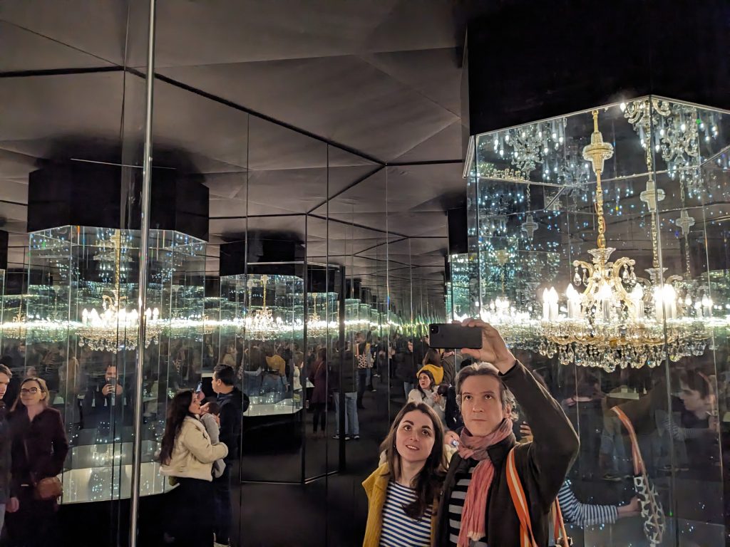
This photo captures my fiancé Lina and myself at Yayoi Kusama’s “Infinity Mirror Rooms” exhibit at Tate Modern in London, taken in March 2024. The installation, called “Chandelier of Grief,” uses mirrors and light to explore ideas about symmetry.
The centrepiece of the artwork is a chandelier surrounded by six mirrors arranged in a regular hexagonal prism. This creates an interesting visual effect—an infinite lattice of chandeliers extending in all directions, with each reflected chandelier appearing at the centre of symmetry within this lattice.
What we’re experiencing is a visual representation of a hexagonal lattice, one of the five two-dimensional Bravais lattices. Mathematically, it represents a discrete group of isometries in two-dimensional Euclidean space. The point group of this hexagonal lattice is isomorphic to the dihedral group  , highlighting its sixfold rotational symmetry and mirror reflection properties.
Physically, the hexagonal lattice emerges as the ground state configuration for systems of particles interacting via certain potentials, such as the Lennard-Jones potential, in the thermodynamic limit. Moreover, the hexagonal lattice is realised in materials like graphene, where carbon atoms arrange themselves in this highly symmetric pattern, leading to its unique properties.
Kusama’s installation is not only aesthetically pleasing but also serves as a visual representation of abstract concepts in mathematics and physics. The infinite reflections illustrate how artistic expression can intersect with scientific principles, making complex ideas accessible and engaging to a wider audience.
 . Here,
  represents the volume of the unit cell
  , and
, and  is the volume of the subset of
  .
.  . However, analytically computing the volume of
 is the natural volume form on
  . Since this integral is zero everywhere except in the unit cell, it can be redefined as an integral of the indicator function over the unit cell:
 , we get:

 as a uniform random vector on the unit cube, this integral represents the expected value of the indicator function with respect to the
  -variate uniform distribution. This, in turn, equals the probability of
  lying in the collection of the van der Waals spheres
  , scaled by the inverse of the unit cell:
![\begin{equation*}$\rho=\textbf{E}\left[ \bm{1}_{\mathbf{U}^{-1}\mathbf{O}} \right]=\text{P}\left( X \in \mathbf{U}^{-1}\mathbf{O} \right)\end{equation*}](https://milotorda.net/wp-content/ql-cache/quicklatex.com-1c0ff9421f08065d4885c3797a231318_l3.png "Rendered by QuickLaTeX.com")
 , counting how many fall inside
  :
:
 anthracene structure
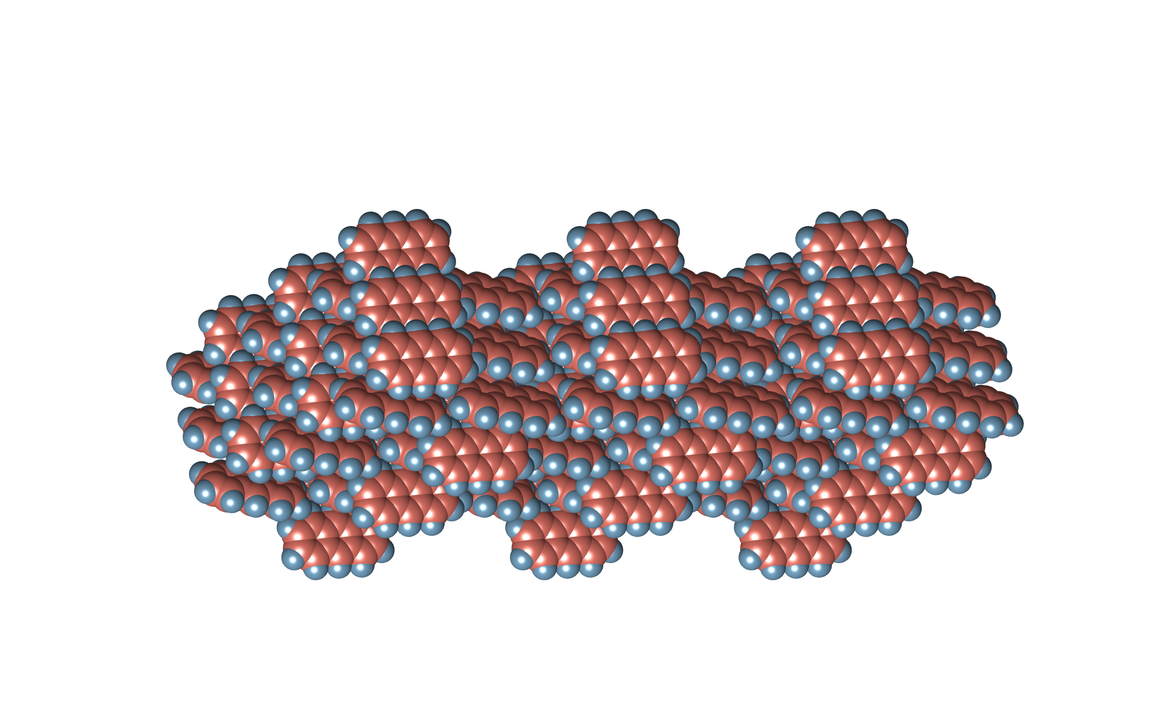
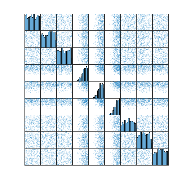
 realisations,
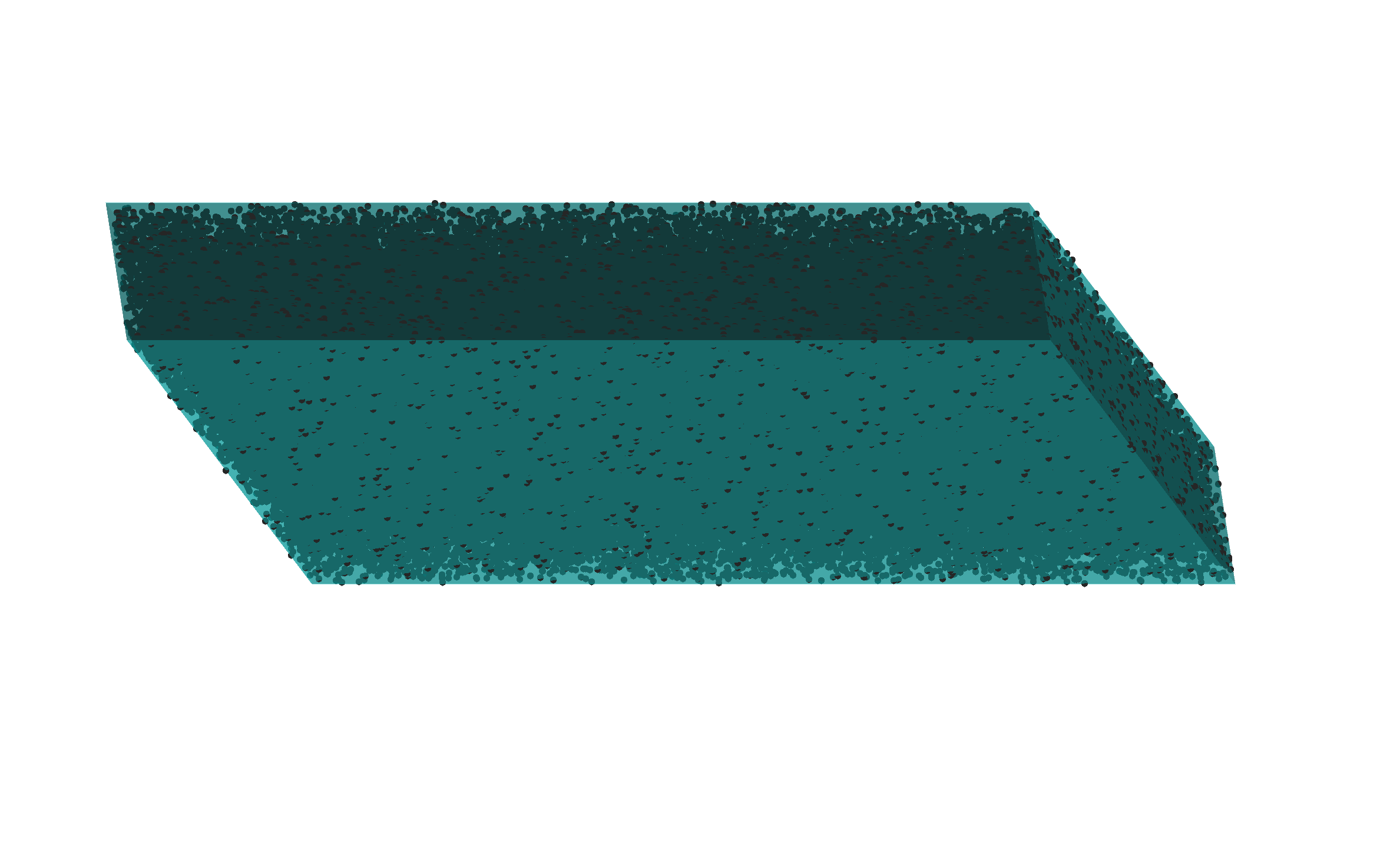
 . Therefore, the density estimate is
  .
. , where
  is some constant?
 as a Bernoulli trial. Then
  is a binomially distributed random variable with the expected value
  and variance
  . According to the central limit theorem, the random variable
  converges in distribution to a normally distributed random variable with a mean of
  and a variance of
  . Therefore, I can request
  being in the interval
  , and I want the size of this interval to be less than some constant with probability
  :
:
 is the
  quantile of the standard normal distribution.
 with probability
  , I need
  . The density estimate in this case is then:
 .
Closing note: This method could also be used to quantify uncertainty about the true packing during
.
Closing note: This method could also be used to quantify uncertainty about the true packing during 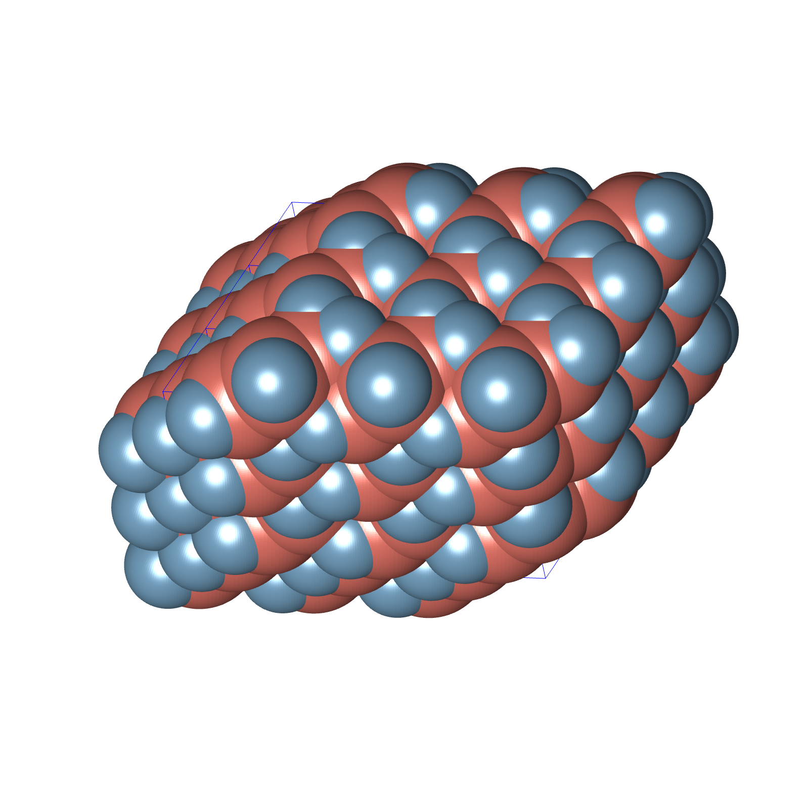


 takes this form:
 .
. represents the mean of all samples in the current batch, and I only consider the configurations without overlap or the repaired ones that lie within the optimization boundaries for
  . This effectively means I’ve eliminated the need for the penalty function and am optimizing only based on the objective function given by the packing density.


 in the tangent space
  of the statistical manifold, where everything is unfolding, but what I actually need is
  in the tangent space at the point
  using this vector
  (where
  to
to  ), and then I compute the natural gradient at the point


 . Previously, reaching such a level of density required multiple rounds of the refinement process, each consisting of
  iterations. Now, a single run with just
  iterations is sufficient. It’s worth noting that even after only
  iterations, the algorithm already reaches areas with densities exceeding
  .
. space group. However, similar repairs can be done for configurations in any space group. Furthermore, the algorithm’s convergence speed can be further enhanced by fine-tuning its hyperparameters. Perhaps it’s time to make use of the BARKLA cluster for the hyperparameter tuning.
![\begin{equation*} E_{LJ}=\sum_{\{ A, B \} } \frac{1}{2}\sum_{a \in A} \sum_{b \in B} 4\epsilon\left[\left(\frac{\sigma}{r_{ab}}\right)^{12} - \left(\frac{\sigma}{r_{ab}}\right)^{6}\right] \end{equation*}](https://milotorda.net/wp-content/ql-cache/quicklatex.com-e667e732de97bd4a1f260d50e3bd9bbb_l3.png "Rendered by QuickLaTeX.com")
 and
and  . Here,
  represents the ordered pair of molecules
  and
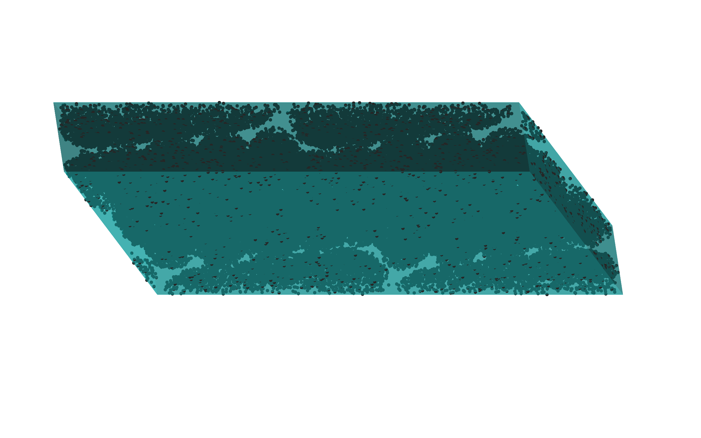
and  . The simulation involves a system of
  molecules, each comprising
  atoms. At the start, a uniform random configuration was generated, with each molecule represented by two center of mass coordinates and one rotational coordinate.
 regular tiling.
 (
( below.
 and
and  with the unit cell given by
![\begin{equation*} U=\left[\begin{array}{ccc} a\sin(\beta)\sqrt{1-\left(\frac{\cos(\alpha)cos(\beta) - cos(\gamma)}{\sin(\alpha)\sin(\beta)}\right)^2} & 0 & 0 \\ -a\frac{\cos(\alpha)cos(\beta) - cos(\gamma)}{\sin(\alpha)} & b\sin(\alpha) & 0 \\ a\cos(\beta) & b\cos(\alpha) & c \end{array}\right] \end{equation*}](https://milotorda.net/wp-content/ql-cache/quicklatex.com-8822e93316b6a3860f7b5ea171f09621_l3.png "Rendered by QuickLaTeX.com")
 equals to
  and combined with the volume of the unit sphere
  gives the optimal packing density of spheres
  . See a visualization of this configuration below.

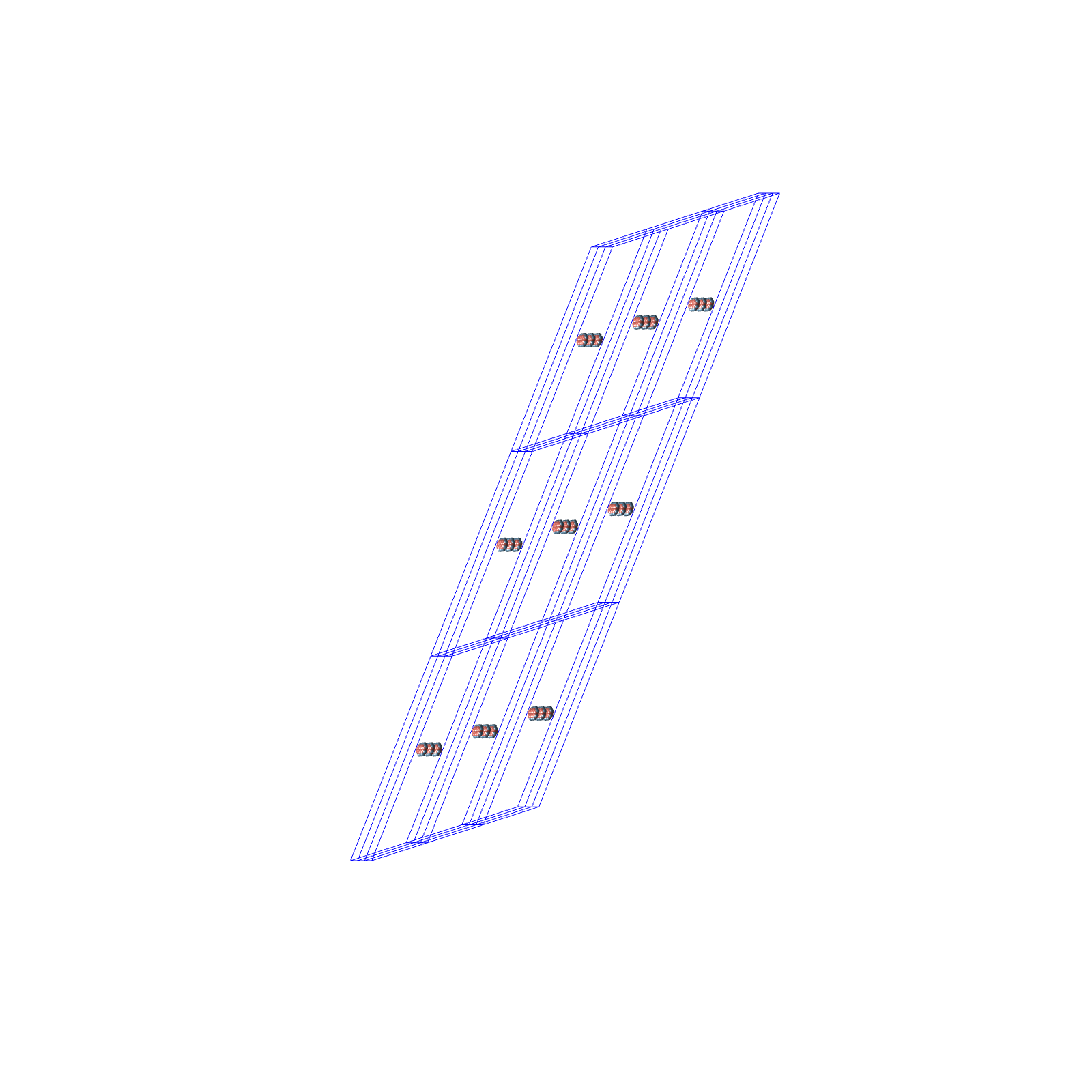
 ,
,  and
and  , then the determinant of the unit cell equals to
  and again we get the optimal packing density of spheres
  . See the visualization of this configuration below.

 ,
,  ,
,  and
and  and again we get the optimal packing density of spheres
  . See the visualization of this configuration below.


