
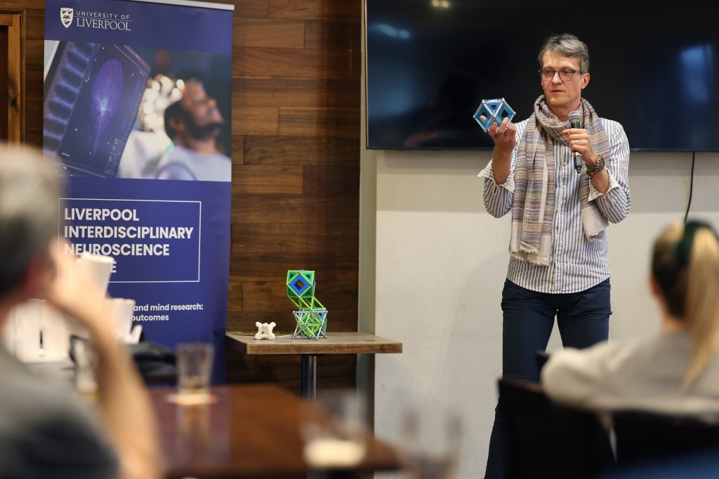
This week I gave a Shots of Science talk — three minutes, no slides, props only, at the Bridewell during the Pint of Science 2026 Neuro-Night . The Shots of Science format: short, punchy talk from a mix of researchers slipped between the evening’s main speakers. The premise alone is an interesting challenge: distill your research into 180 seconds for a science-curious pub audience.
The talk was an attempt to take one piece of my research — the densest packings of cuboctahedral molecules — and shrink it to a single mystery tour you could hold in one hand. A useful exercise in Richard Hamming’s Importance test: can you “paint a general picture to say why it [your research] is important”?
What the talk says
Picture a greengrocer’s stall: a neat pyramid of oranges. Why a pyramid? Because round things are very good at finding the gaps. Each orange nestles into the little hollow between four below it. Cannonballs do it. Snowflakes do it. In the best case, about three quarters of the space is fruit; the rest is tiny pockets of air.
But molecules are not always round.
What if your orange isn’t an orange? What if it’s a tiny cage of atoms, hollow in the middle, made from triangles and squares? Chemists can make cage-like molecules, and if we want to turn them into useful materials, we need to ask the old cannonball question again: how do they stack?
So I did the obvious thing. I built the prettiest, most regular arrangement I could. It looked beautiful. It looked logical. It looked right. Then I used a computer to search the promising crystal patterns. And the answer was: no. The pretty one comes second.
The winner is awkward. Tilted, lopsided, much less regular. But the holes and bumps cooperate — and this hollow molecule still packs nearly as tight as those cannonballs. Twelve of the thirteen spheres are there; only the middle one is missing.
That matters because crystals are made by molecules choosing neighbours. And it isn’t just toys — chemists are building real molecules that look like this. Most crystals chemists have ever measured fall into just a handful of these repeating arrangements — four out of every five. If we know which shapes like to fit, we can begin with the material we want and ask what kind of molecule might build it.
And the bit I love is this: this researcher’s brain wanted the neat answer. The geometry chose the awkward one. Nature does not always pick the prettiest arrangement. Sometimes the lopsided one wins.
The props
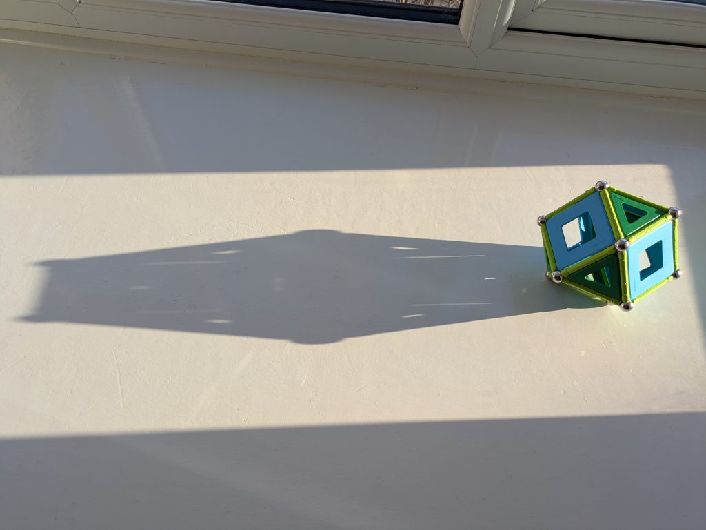
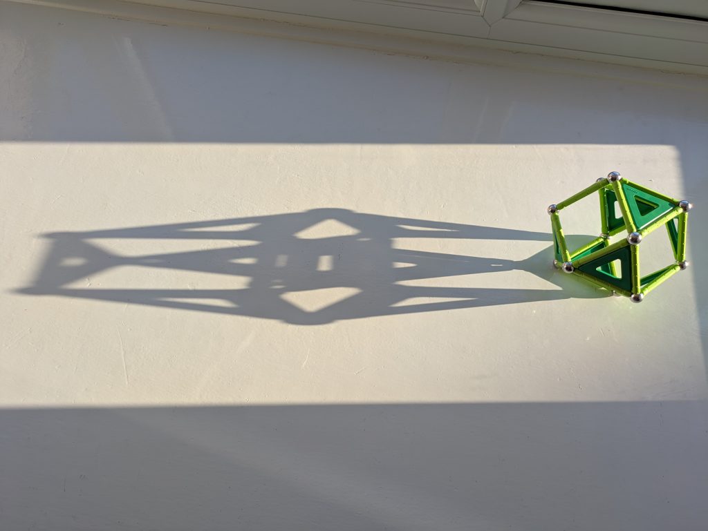
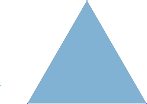
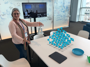
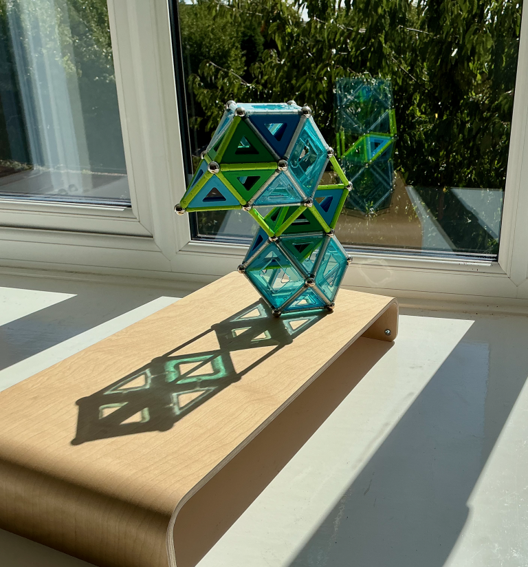
Four objects sat on the small table. The cuboctahedron I’m holding in the photo above is a GEOMAG model: twelve magnetic vertices arranged on the corners of the polyhedron, eight triangular faces and six square ones. It is the geometric idea of the talk — what a single cuboctahedral molecule “looks like” if you strip everything except the shape.
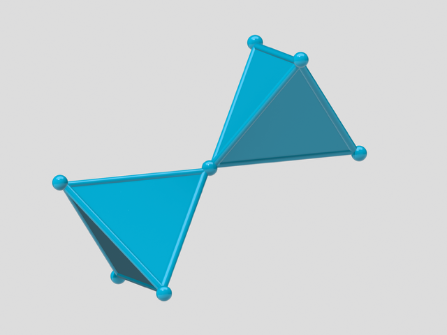
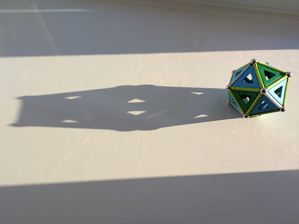
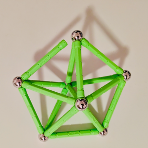
The white object on the table is a 3D print of a real cage molecule, bumpy with its printer layer-lines, lighter and more fragile than the magnetic models. It is the same family of geometry made concrete — a reminder that real chemists really do make molecules like this. Between both handled props sat Kepler’s stella octangula: two interpenetrating tetrahedra whose eight vertices sit on the eight corners of a cube — eight of the lattice positions of the FCC arrangement that the script names in the hook (the cube’s six face-centres are the rest of the regular orange stack). And on the back row of the table sat the green-and-blue magnetic model of a single tetrahedral-octahedral honeycomb cell — a fragment of the lopsided crystal, made tactile.
The Prime Radiant Easter egg
The GEOMAG cage I’m holding is the same shape Apple TV’s Foundation (2021–) chose for the Prime Radiant — the handheld geometric object Hari Seldon uses to encode the mathematical laws by which civilisation rises and falls. Buckminster Fuller called it the ‘vector equilibrium’ — a natural choice for an object that wants to look like it holds the geometry of everything.
Thank you
Thanks to Pint of Science Liverpool for inviting me, and to Melissa and Rosie for organising the night. And to my wife Lina, in the front row, for support: the cuboctahedral packing in this talk is also the configuration in a Valentine GIF I made for her earlier this year. Sometimes the lopsided one wins.
If you want the maths behind any of this, the full research blog post — Densest Packings of Cuboctahedral Molecules — has the figures, the space groups, and a 12-of-13 spheres argument for the global maximum.
 Cuboctahedral Molecule Packing
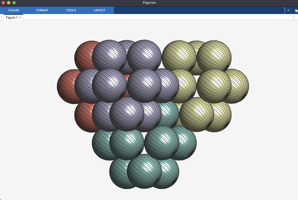
 framework of


 . See the densest packing configuration found during one optimisation run of the molecular packing algorithm’s search in the space group


 . Since the volume of our tetrahedral molecule is
  (4 times the volume of a sphere with radius
  ), according to the geometric packing density formula
  and the number of elements of factor group
  where
where  is the lattice subgroup of
  , is
, is  ,
,  which is exactly the density of FCC close-packing of equal spheres.


 wallpaper group. Now if we fold up the this group by identifying the symmetry elements we end up with a surface akin to a sphere containing four
 orbifold with a circle and thus creating a “fibered orbifold” or a
  . The primary fibrifold name of space group
  .
.


 and
and  with orbifold names
  and
and  respectively.


 with the fibrifold name
  and
and  .
.
 (orbifold name
  ), reflected in the

 with its fibrifold name
  and
and  with its fibrifold name
  to our list.
 (orbifold name
  ) square tiling symmetry in one of the tetrahedral molecular packing special projections.


 . Its fibrifold name is
  .
.
![\[ \begin{tabular}{ll|ll|ll|ll} \hline \hline \multicolumn{8}{c}{\textbf{Symmetries of the} $\mathbf{P\bar{1}}$ \textbf{Tetrahedral and Octahedral Molecule Packings}} \\ \hline \multicolumn{2}{c|}{\textbf{Closest-Packed Space Groups}} & \multicolumn{6}{c}{\textbf{Symmetries of Special Projections}} \\ \hline \textit{H-M} & \textit{Fibrifold (primary)} & \textit{H-M} & \textit{Orbifold} & \textit{H-M} & \textit{Orbifold} & \textit{H-M} & \textit{Orbifold} \\ \hline $P\overline{1}$ & (2 2 2 2) & $p2$ & 2 2 2 2 & $p2$ & 2 2 2 2 & $p2$ & 2 2 2 2 \\ $P2_{1}$ & ($2_{1} 2_{1} 2_{1} 2_{1}$) & $pg$ & $\times \times$ & $pg$ & $\times \times$ & $p2$ & 2 2 2 2 \\ $P2_{1}/c$ & ($2_{1} 2_{1} 2 2$) & $p2mg$ & 2 2 * & $p2gg$ & 2 2 $\times$ & $p2$ & 2 2 2 2 \\ $C2/c$ & ($2_{0} 2_{1} 2 2$) & $c2mm$ & 2*2 2 & $p2mg$ & 2 2 * & $p2$ & 2 2 2 2 \\ $P2_{1}2_{1}2_{1}$ & ($2_{1} 2_{1} \overline{2}$) & $p2gg$ & 2 2 $\times$ & $p2gg$ & 2 2 $\times$ & $p2gg$ & 2 2 $\times$ \\ $Pbca$ & ($2_{1} 2\overline{*} :$) & $p2mg$ & 2 2 * & $p2mg$ & 2 2 * & $p2mg$ & 2 2 * \\ \hline \end{tabular} \]](https://milotorda.net/wp-content/ql-cache/quicklatex.com-7feaf7092df8b1622f700599e7a496b2_l3.png "Rendered by QuickLaTeX.com")
 and
and  Tetrahedral Molecule Packings
 and
and 


 .
.


 and
and 


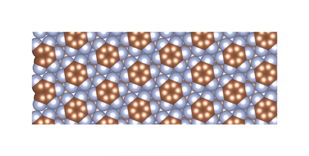
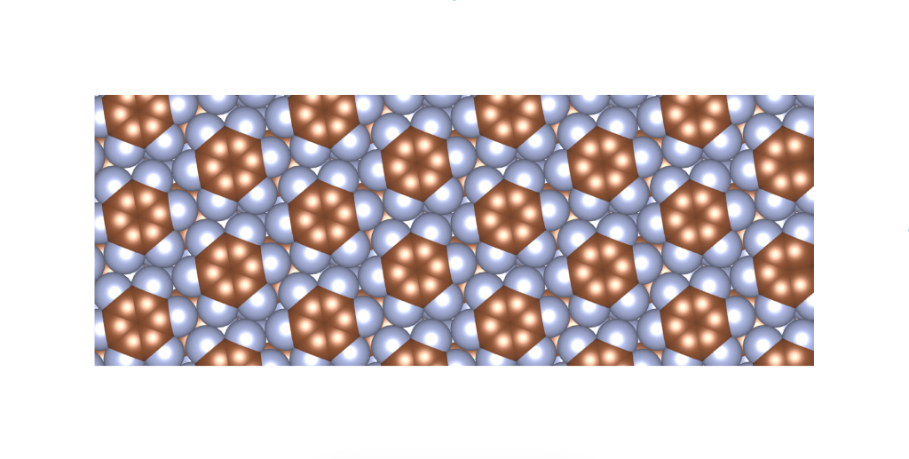
 , which is the second densest cuboctahedral molecule packing in our list. Have a look at the comparison between the GEOMAG model and the structure from our computational experiment.


 . The GEOMAG model representing this arrangement appears like this:


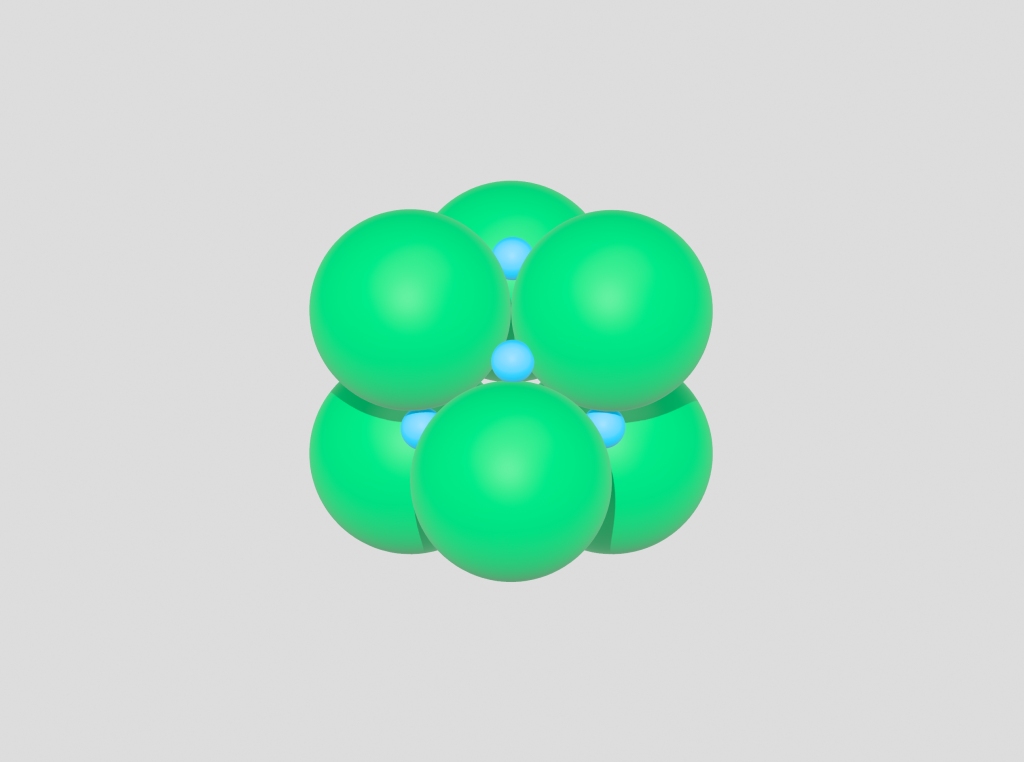
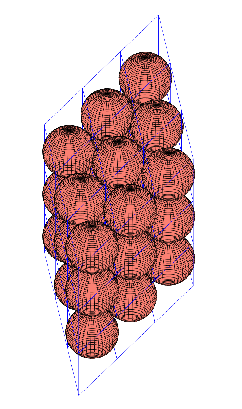
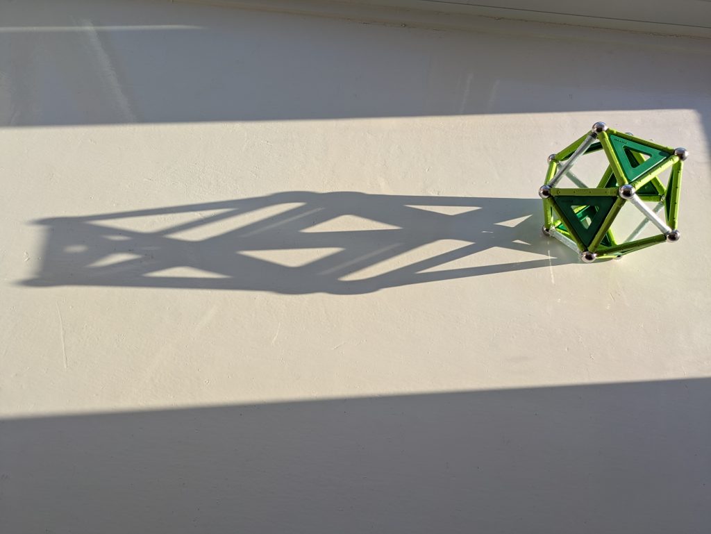
 short of the densest packing of equal spheres, and by construction our cuboctahedral molecule model is a collection of equal spheres with centres on the twelve vertices of a cuboctahedron, missing exactly one sphere on the inside. Conversely, the twelve spheres are in the densest possible arrangement around a single one—or shall we say—in the vector equilibrium of
  packing — as shown in the image on the left below.


 ,
,  ,
,  ,
,  ,
,  , and
, and  , which is the full symmetry of the face-centred cubic lattice.

 . See
. See 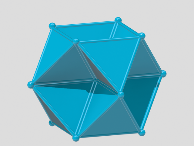
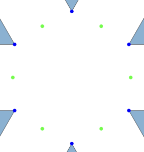
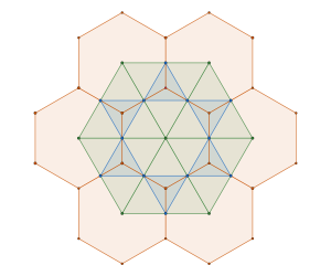
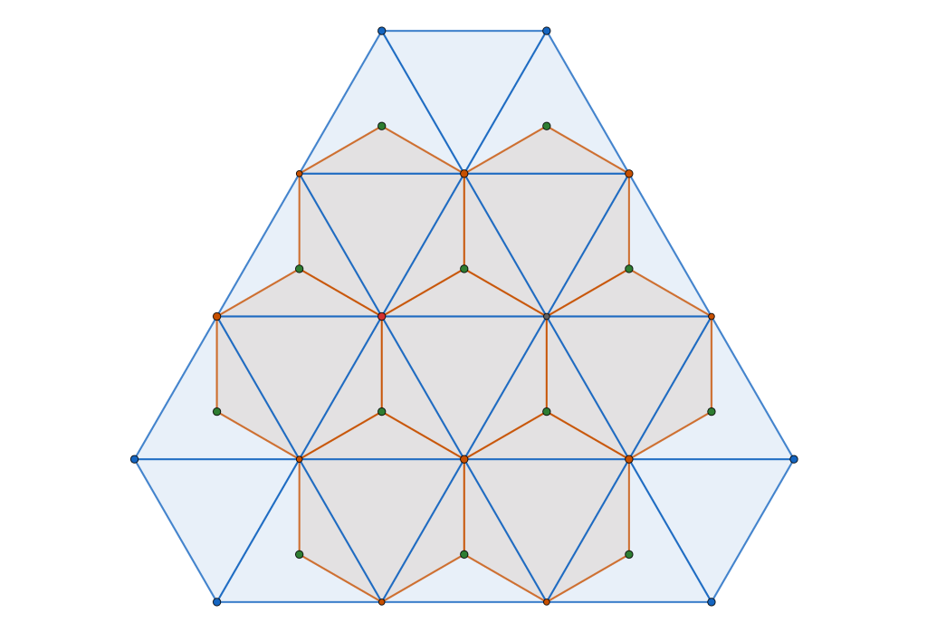
 ) and green (
 ) charged particles that satisfies this criterion under the Coulomb potential.

![\begin{equation*} C_0 = \text{argmin}_{\iota:C_0 \rightarrow \mathbb{R}^{2k}} \left[ E^{C}(C_0^{\iota}) \right]^2 \end{equation*}](https://milotorda.net/wp-content/ql-cache/quicklatex.com-fbe580ac2647632148f2224fd5efe19d_l3.png "Rendered by QuickLaTeX.com")
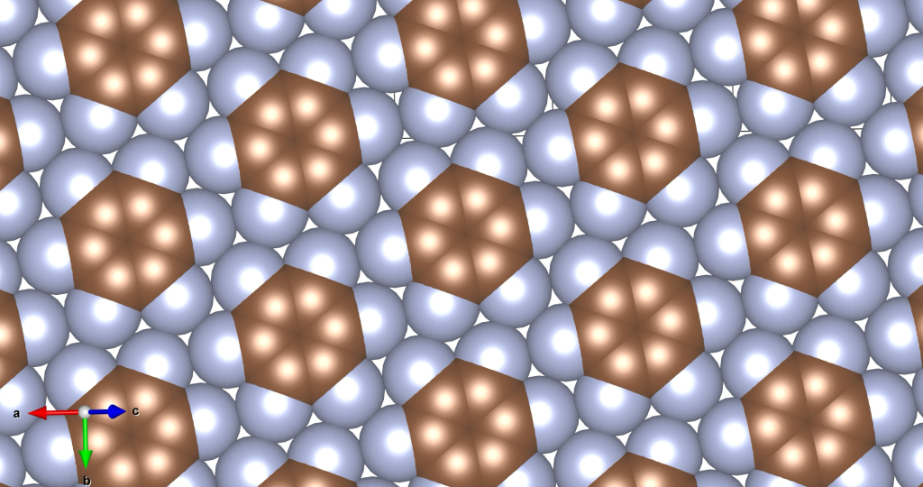
 ). The similarity is not merely mathematical; chemically, the tetrahedral framework model could approximate a real organic
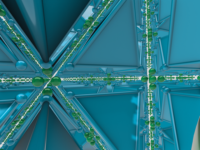
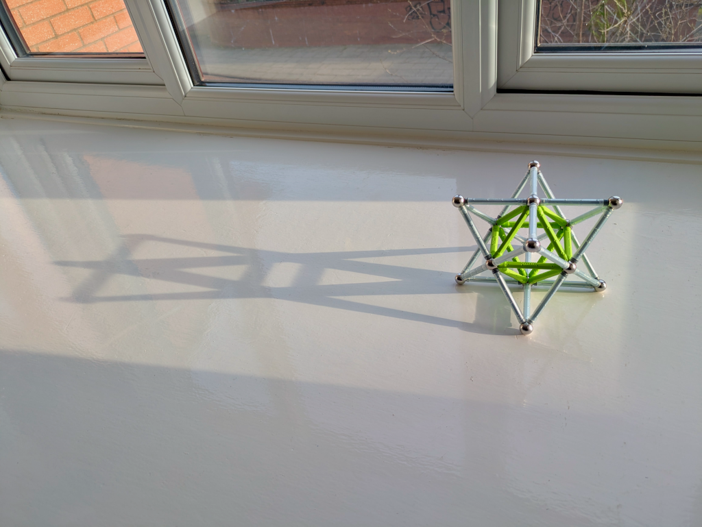
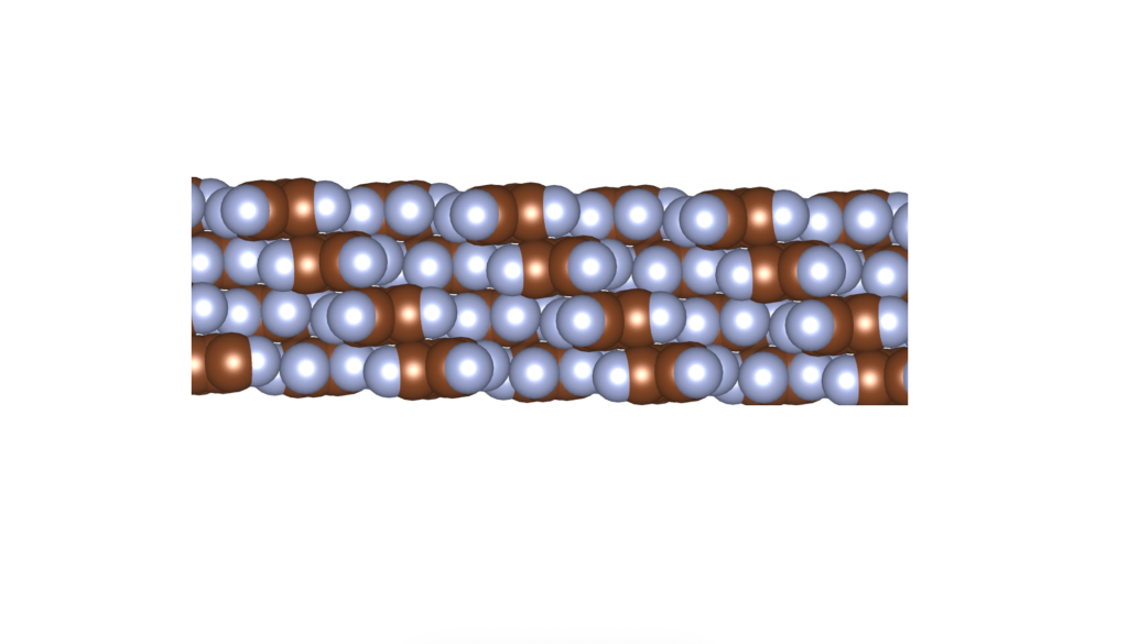
 (space group 227), same as diamond, and it is mechanically quite stable, as shown in the photo below.

 (space group 224).
 -subgroup of


 and
and  denote molecules of either type (green negative or blue positive triangular),
  is the Euclidean distance between charges
  and
and  . For green particles,
  , while for vertices of blue triangles,
  . This creates attractive forces between opposite charges and repulsive forces between like charges, proportional to their relative distance.
 between molecules
 where the following limit converges to a constant:

 represents a collection of
  molecules of both types (
 ).
).
 , an alternating configuration of charges in a local cluster can found for any
  . Moreover, due to the rigidity of triangular molecules and the form of the potential
  , the maximal cluster contains
  charges.
 , we set the energy to:

![\begin{equation*} C_0 = \text{argmin}_{\iota:C_0 \rightarrow \mathbb{R}^{2k}} \left[ E^{C}(C_0^{\iota}) +1 \right]^2 \end{equation}](https://milotorda.net/wp-content/ql-cache/quicklatex.com-3e7577ae5bfe3cd94d7847e44f750a29_l3.png "Rendered by QuickLaTeX.com")
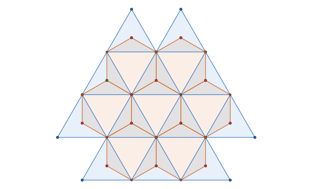
 configuration, the blue positive charges occupy the
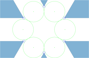

 is an index set . Minimizing
  for such a cluster collection becomes a well-defined problem:

 , the solution is illustrated below.
 respects molecular memberships—for
  and
and  , we require
  .
.
 to
to  :
:
 .
.
 for
for  , and we already know that the global minimizer is a dilated, translated, or rotated version of the triangular lattice.
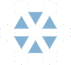
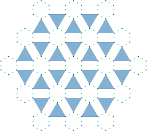
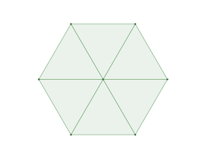
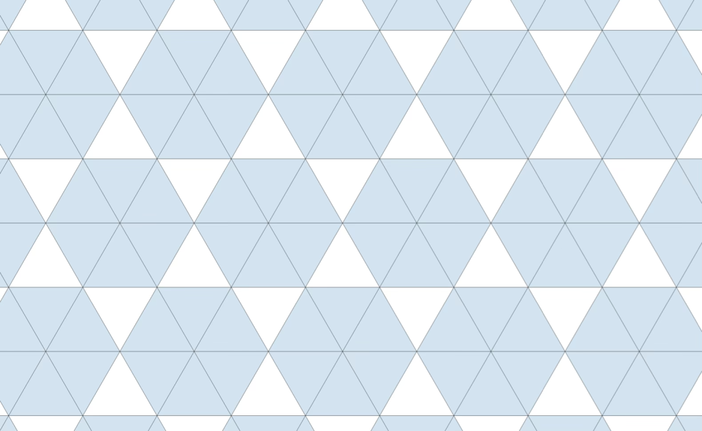
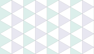
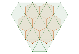
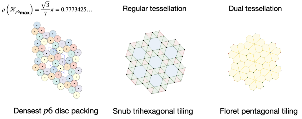
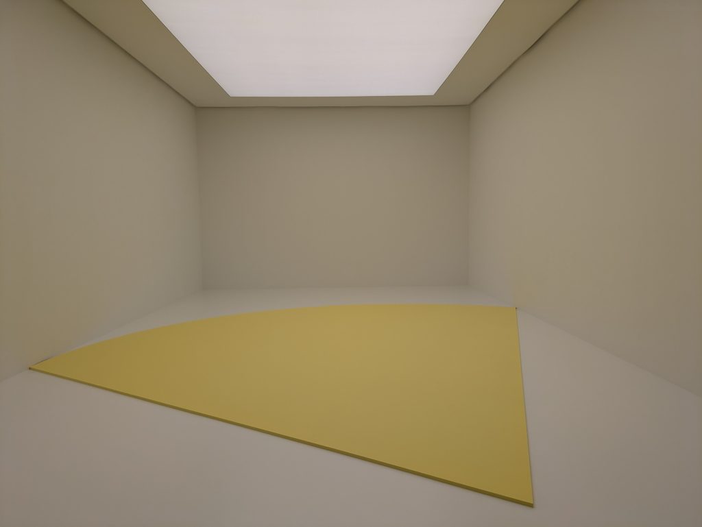
 configuration with a density of
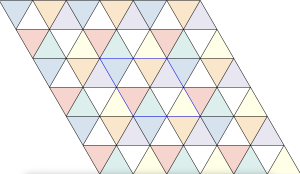
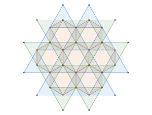
  . It is, in fact, a tiling of triangles as shown below.
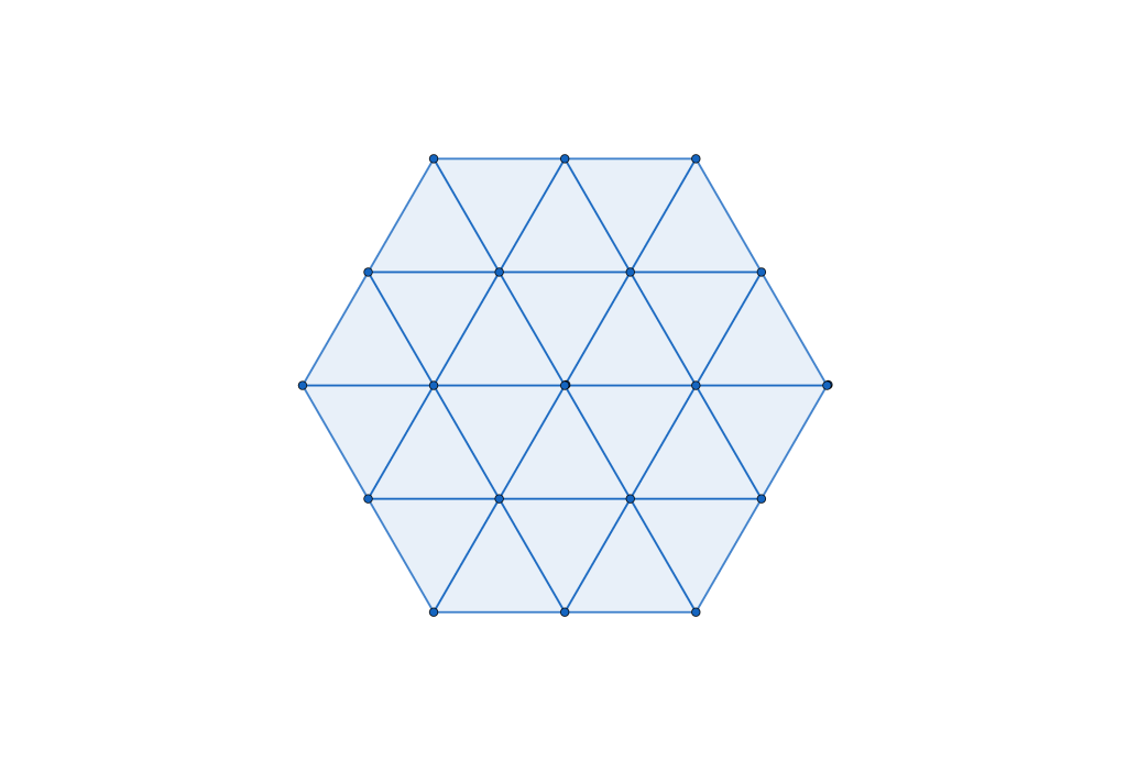
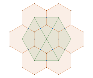
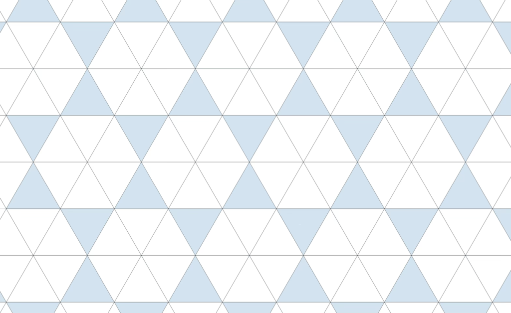
 plane group. The densest packing of regular triangles when the packing configurations are restricted to the
  and is shown in the image below.


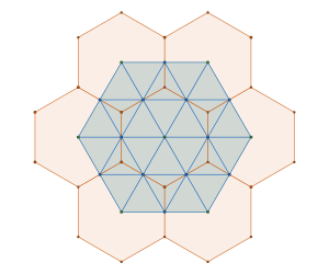
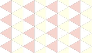
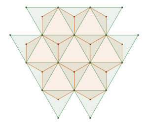
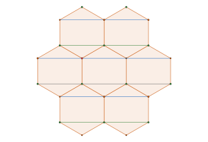
 is constructed by removing triangle tiles containing a vertex at its center of mass
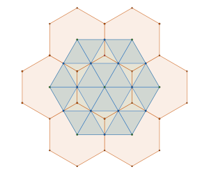
 by removing tiles not containing an interior vertex
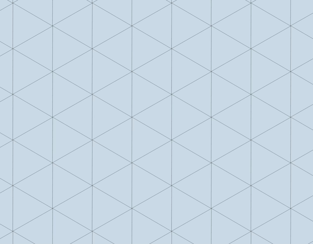
 triangle packing which is in fact a tiling
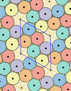

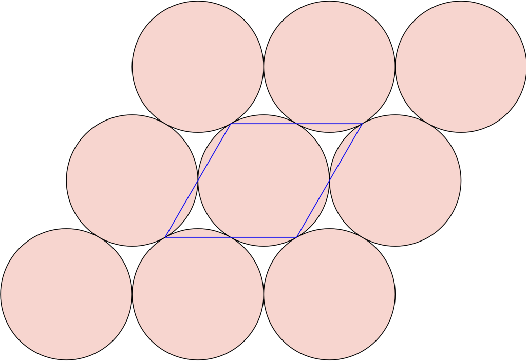
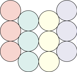
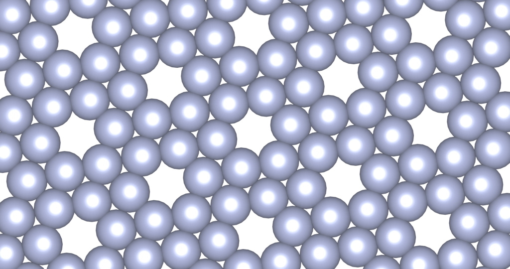
 packing of discs
 with respect to zero (center of the middle pentagon).

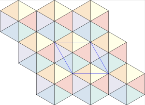
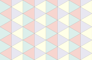
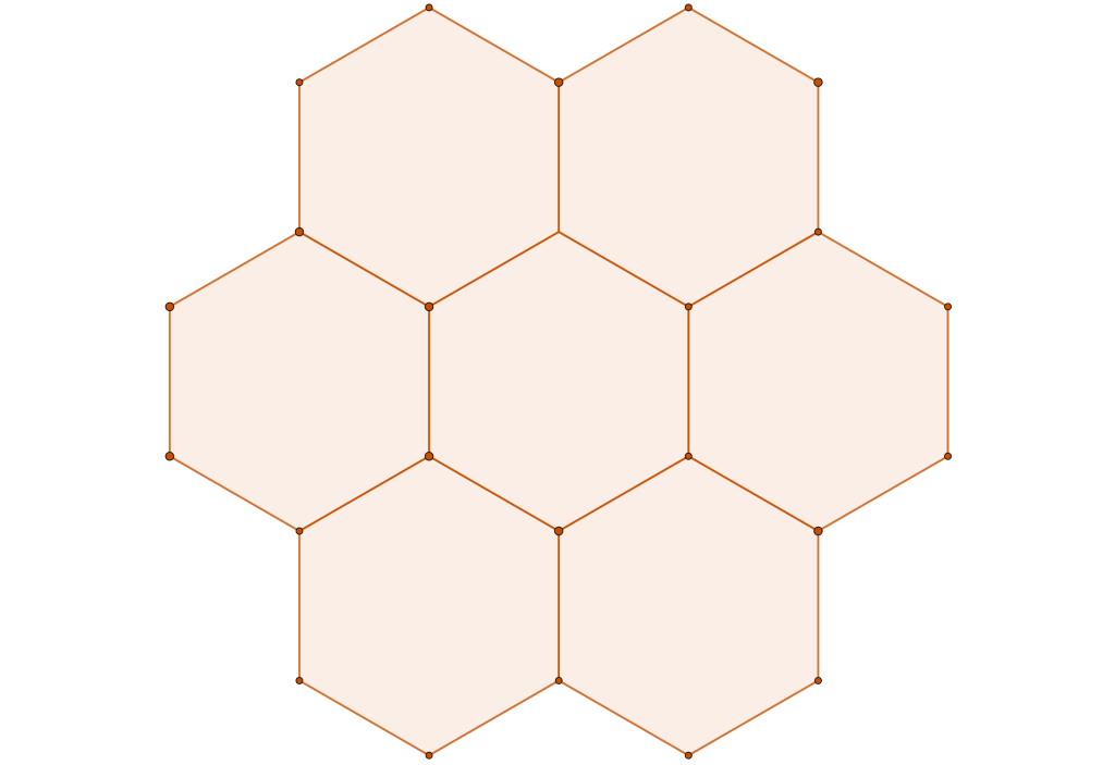
 semi-regular tiling
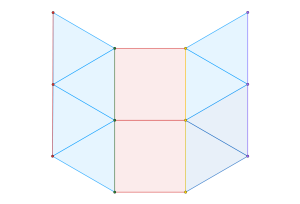
 , of regular
  -gons meet at each vertex. In triangular tessellations, six regular triangles (
 -gons) meet at each vertex. For regular tessellations like the triangular one, this follows a simple equation:

 regular
  -gons (triangles) and
  regular
  -gons (squares).
 , there exists at least one
  such that the expression
  holds. Thus, for any such
  tends to infinity, the

![\begin{equation*} E_{LJ}=\sum_{\substack{\{I,J\} \\ I \cap J =0}} \sum_{\substack{(i,j ) \\ i \in I, j \in J}} \left[\left(\frac{1}{r_{(i,j)}}\right)^{12} - \left(\frac{1}{r_{(i,j)}}\right)^{6}\right] \end{equation*}](https://milotorda.net/wp-content/ql-cache/quicklatex.com-562681f5736399b7414a50ca69c95723_l3.png "Rendered by QuickLaTeX.com")
 is the Euclidean distance between the
  -th atom of molecule
  -th atom of molecule
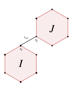
 minimization problem.
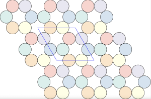
 packing of discs. This means that there are also two chiral densest
  packings of all
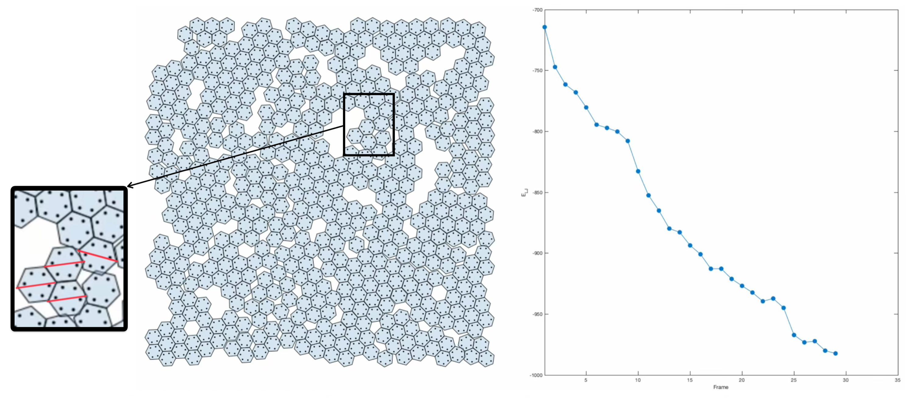
 and
and  group. Even though they belong to different crystal systems—triclinic for
  ,
,  , and
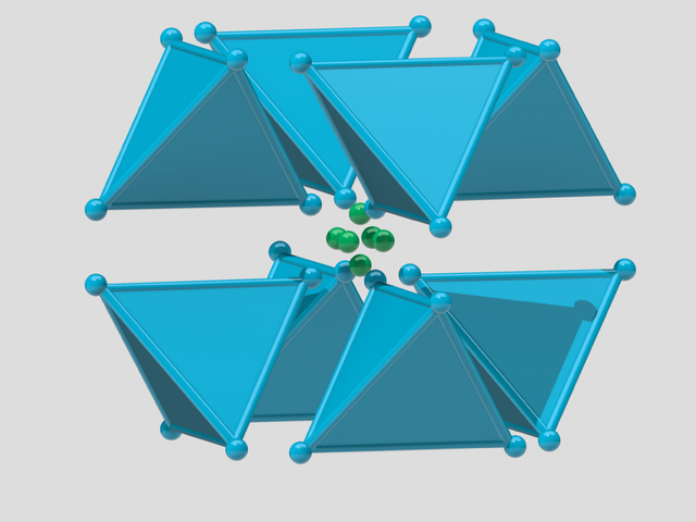
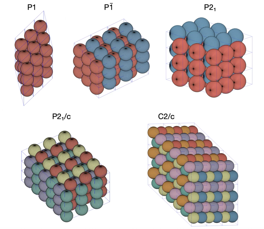
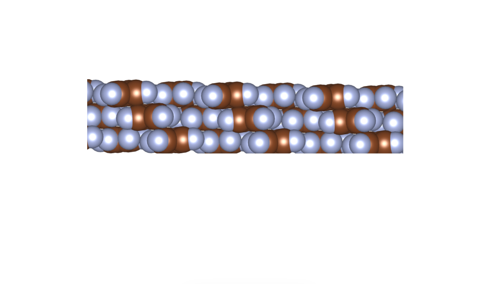
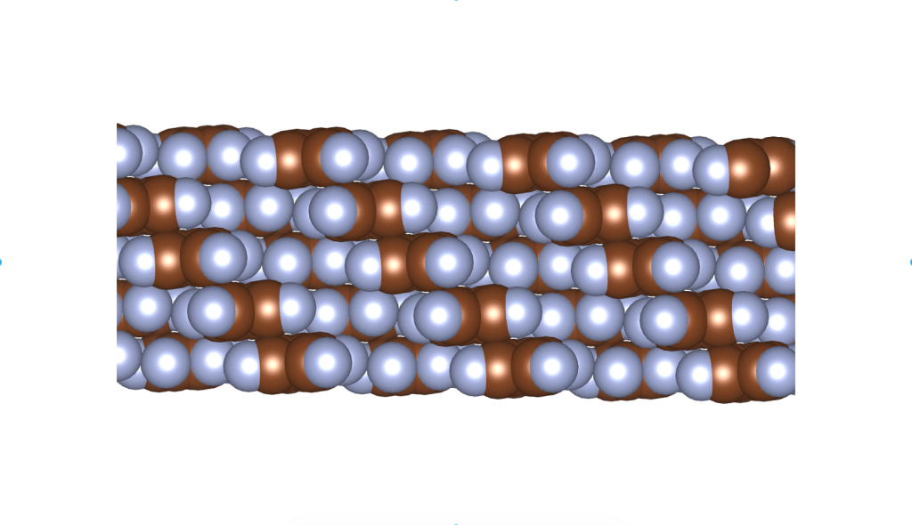
, and  . Here’s a snapshot of what this packing looks like:
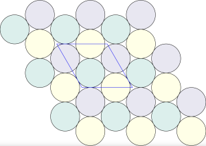
 ,
,  , and
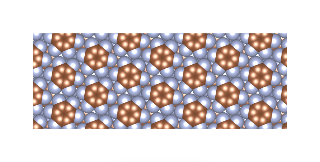
, and  . Check out the illustration below of the densest packing configuration:
 ,
, 