Repairing Unfeasible Solutions in ETRPA.

The ETRPA is designed to optimize a multi-objective function by:

1. Maximizing packing density.
2. Minimizing overlap between shapes in a configuration.

This is achieved through the use of a penalty function, which generally works quite effectively. However, there are some downsides to this approach. Many generated samples are flagged as unfeasible, leading to inefficiency. Additionally, some potentially good configurations with minimal overlaps are discarded. A more effective approach would involve mapping unfeasible solutions to feasible ones, essentially repairing the overlaps.

I’ve designed a relatively straightforward method to accomplish this almost analytically. It boils down to finding roots of a second-order polynomial, which is essentially a high school algebra problem. Admittedly, you’ll need to solve quite a few of these second-order polynomials, but they are relatively easy to handle.

So, with this approach, you can now map a configuration with overlap/s

to one without overlaps

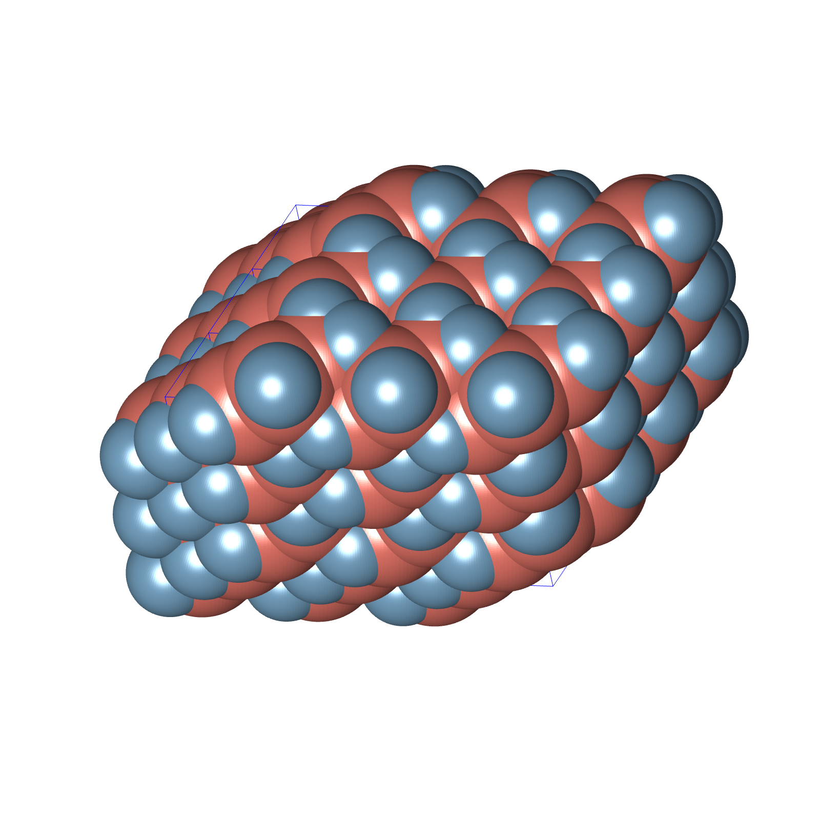
Now, a couple of new issues have cropped up. First, there are some seriously bad solutions that are being sampled. For example, consider this one:

which is then mapped to this configuration

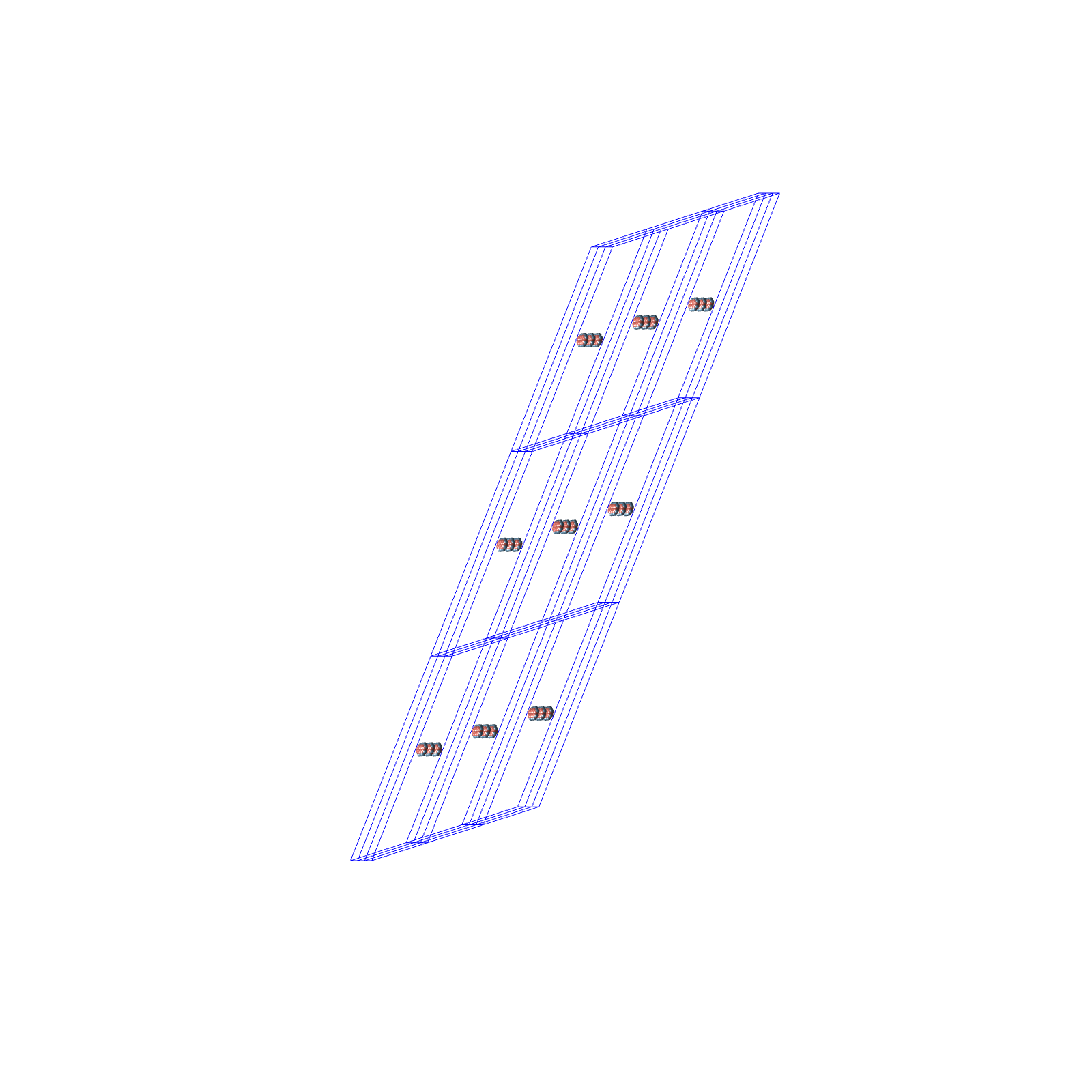
This is not helpful at all. Second, the parameters of this configuration are way above the optimisation boundaries that were used to create all configurations. As a result, it falls outside the configuration space where my search is taking place.

To address this issue, after repairing the configuration, I conduct a check to determine if the repaired configuration falls within my optimization boundaries. Any configurations that fall outside of these bounds are labeled as unfeasible solutions.

It might seems this puts me back in the same situation of multi-objective optimization, but that’s not the case. In my scenario, the Euclidean gradient at time $t$ takes this form:

$\nabla_{\bm{\theta}} J(\bm{\theta}^t) \ = \ \bm{\mu}^t_{\textbf{F}_{1- \frac{1}{q^{*}}}}-\bm{\mu}^t$ .

Here, $\bm{\mu}^t$ represents the mean of all samples in the current batch, and I only consider the configurations without overlap or the repaired ones that lie within the optimization boundaries for $\bm{\mu}^t_{\textbf{F}_{1- \frac{1}{q^{*}}}}$ . This effectively means I’ve eliminated the need for the penalty function and am optimizing only based on the objective function given by the packing density.

This is a promising, but it does introduce another problem. When I repair some of the unfeasible configurations, I end up making slight alterations to the underlying probability distribution, shifting it slightly from $\bm{\theta}^t$

to $\bm{\theta}_{\text{rep}}^t$

The issue here is that if I were to compute the Natural gradient as I used to, I’d obtain $\widetilde{\nabla} J(\bm{\theta}_{\text{rep}}^t) =\mathcal{I}_{\bm{\theta}_{\text{rep} }^t}^{-1} \left({\bm{\mu}_{\text{rep}}^t}_{\textbf{F}_{1- \frac{1}{q^{*}}}}-\bm{\mu_\text{rep}}^t\right)$ in the tangent space $\mathcal{T}_{\bm{\theta}_\text{rep}^t}$ of the statistical manifold, where everything is unfolding, but what I actually need is $\widetilde{\nabla} J(\bm{\theta}^t)$ in the tangent space at the point $\bm{\theta}^t$ .

Fortunately, the statistical manifold of the exponential family is a flat Riemannian manifold. So, first, I move from $\bm{\theta}^t$ to $\bm{\theta}_{\text{rep} }^t$ using this vector $\mathcal{I}_{\bm{\theta}^t}^{-1} \left(\bm{\mu_\text{rep}}^t-\bm{\mu}^t\right)$ (where $\bm{\mu}^t$ corresponds to the dual Legendre parametrization of $\bm{\theta}^t$ , and $\bm{\mu}_\text{rep}^t$ to $\bm{\theta}_\text{rep}^t$ ), and then I compute the natural gradient at the point $\bm{\theta}_\text{rep}^t$ .

In addition, to increase the competition within my packing population, I introduce a sort of tournament by retaining the N-best configurations I’ve found so far and incorporating them with the repaired configurations from the current generation. This leads to yet another slightly modified distribution, $\bm{\theta}_\text{rep + N-best}^t$

and I have to perform the same Riemannian gymnastics once more. In the end, the approximation to the natural gradient at the point $\bm{\theta}^t$ is as follows

$\widetilde{\nabla} J(\bm{\theta}^t)$ $=$ $\mathcal{I}_{\bm{\theta}_{\text{rep + N-best} }^t}^{-1} \left({\bm{\mu}_{\text{rep + N-best}}^t}_{\textbf{F}_{1- \frac{1}{q^{*}}}}-\bm{\mu}_{\text{rep + N-best} }^t\right)$ $+$ $\mathcal{I}_{\bm{\theta}_{\text{rep} }^t}^{-1} \left(\bm{\mu}_{\text{rep + N-best}}^t-\bm{\mu_\text{rep}}^t\right)$ $+$ $\mathcal{I}_{\bm{\theta}^t}^{-1}\left(\bm{\mu_\text{rep}}^t-\bm{\mu}^t\right)$

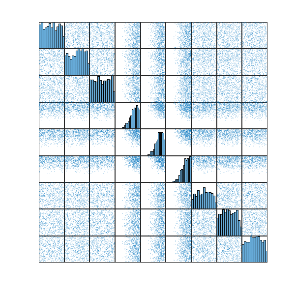
So far, experiments show that these modifications to the ETRPA are far more effective than the original ETRPA. Here’s a visualization from one of the test optimization runs:

In this particular run, the best packing I achieved attains the density of $0.7845$ . Previously, reaching such a level of density required multiple rounds of the refinement process, each consisting of $8000$ iterations. Now, a single run with just $2000$ iterations is sufficient. It’s worth noting that even after only $200$ iterations, the algorithm already reaches areas with densities exceeding $0.7$ .

It’s important to mention that currently, I’ve only implemented the repair process for unfeasible configurations for the $P1$ space group. However, similar repairs can be done for configurations in any space group. Furthermore, the algorithm’s convergence speed can be further enhanced by fine-tuning its hyperparameters. Perhaps it’s time to make use of the BARKLA cluster for the hyperparameter tuning.