To be honest, saying that I made the GIF is a bit misleading. It was actually created by the OpenCode AI coding agent, running the Claude Opus 4.6 model provided by Anthropic. I merely supplied the MATLAB FIG-file of the configuration’s figure, the shape of which reminded me of the heart symbol.
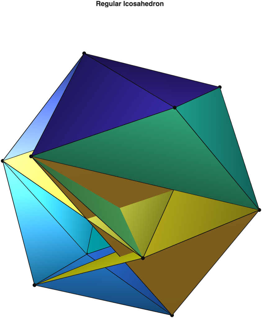
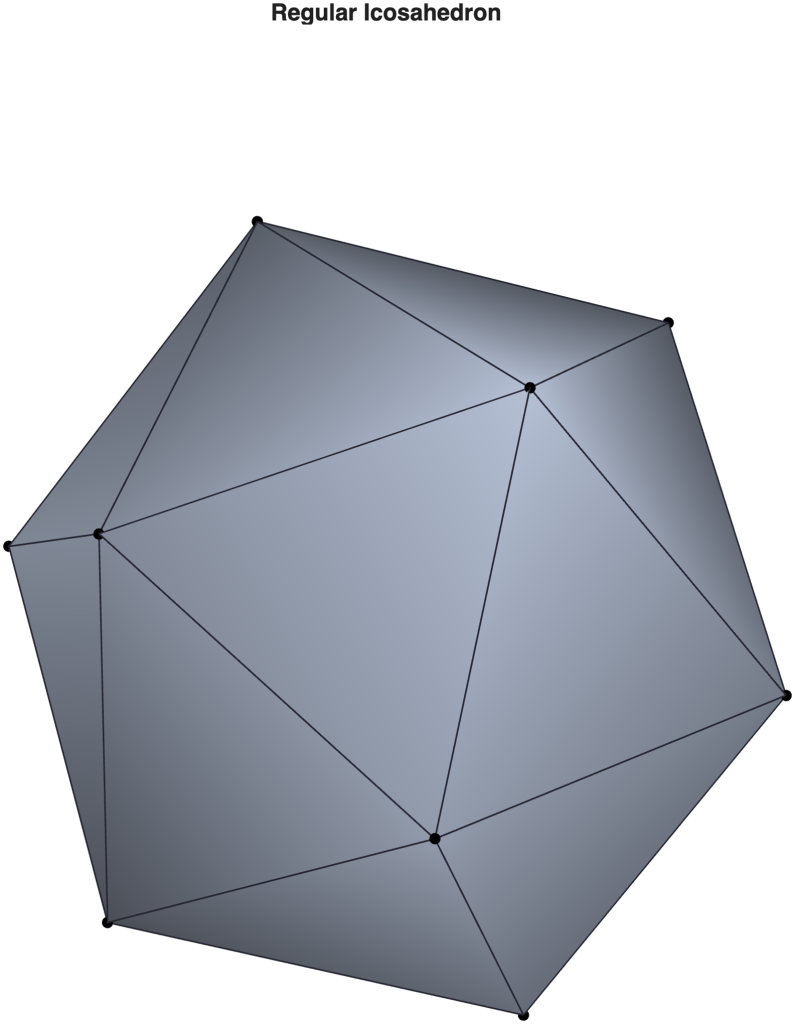
I have been watching closely AI-assisted software development for some time now, but all of the Large language models have proven entirely inadequate for the level of array programming capability required in my research. They have all failed, even at simple tasks such as writing a MATLAB script to visualise a regular icosahedron. For example, below is a response by OpenAI’s state‑of‑the‑art GPT model produced only last September, alongside what an actual regular icosahedron looks like for comparison. You can probably guess which figure is the output of the script written by GPT.
However, a few weeks ago, during my monthly routine check of the state of AI coding assistants, I was genuinely impressed with the framework of Claude Code CLI.
Today, I discovered that MathWorks has already released an official MATLAB Model Context Protocol (MCP) for agentic AI workflows. So I decided to test it thematically on a Valentine animation task. You can see the result at the top of the page.
Solving the task wasn’t as straightforward as I had thought it would be. The main issue lay in getting the orbit of rotation of the camera around the configuration right, but that was more of a mistake on my part, as I didn’t know how to explain it to the agent properly. The initial cycle went surprisingly well. And yes, although it may seem as though the camera is fixed and the object rotates around its axis, it is in fact the object that is fixed, while the camera and the light source rotate around it. It turned out to be easier this way.
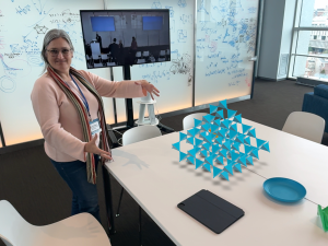
After few back-and-forth exchanges with the agent, once I was satisfied, I asked the agent to create a public repository on my GitHub account, complete with everything needed to generate the animation, including writing a README.md documentation featuring a GIF animation at the top of the page. The result is available here: milotorda-net/cuboctahedral-heart. I’m quite happy with how it worked out.
Now that I have everything set up, it is time to get down to real business with my MATLAB‑context‑armed OpenCode agent.
Last week, I visited Saint‑Malo, France, and presented a poster at the 7th International Conference on Geometric Science of Information, outlining our work on the application of the close‑packing principle to molecular crystal structure prediction. The theme of the 2025 edition of GSI was
From Classical to Quantum Information Geometry: Geometric Structures of Statistical & Quantum Physics, Information Geometry, and Machine Learning.
The poster title and abstract are shown below.
Title: Geometric Modelling in the Prediction of Molecular Crystal Structures: The Close‑Packing Principle Revisited
Abstract: A. I. Kitaygorodsky’s Close‑Packing Principle states that “the mutual arrangement of the molecules in a crystal is always such that the ‘projections’ of one molecule fit into the ‘hollows’ of adjacent molecules,” highlighting the underlying geometries of molecular interactions in crystalline ground states. We revisit this principle to demonstrate that a geometric approach can substantially reduce the computational effort required to predict stable phases of molecular crystals. By leveraging the duality between lattice energy and packing density via a crystallographic space‑group‑induced, geometric-fibrifold constrained programming approach, we generate first‑approximation structures during the initial stages of crystal structure prediction (CSP) within minutes on a standard laptop. Focusing on close packings of volumetric molecular models—where interactions are predominantly van der Waals forces, without any charge or electron exchange—we apply this purely geometric method to various rigid organic molecules. Our results show that integrating the Close‑Packing Principle as a geometric prior reduces computational costs in CSP workflows, enabling more efficient and accurate predictions of molecular crystal structures and promoting ethical and sustainable materials discovery.
Supplementary materials, including the poster handout, are available via the link below.
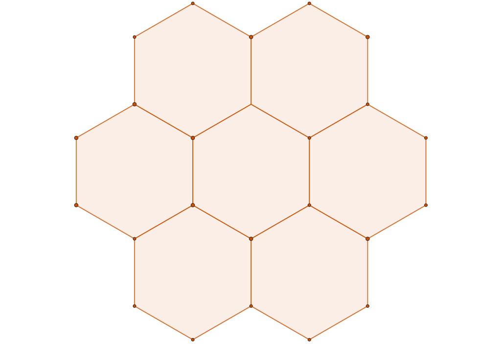
Following up on the packing of the two-dimensional hexagonal molecules in the post Chiral Interaction Energy Ground States, from the materials science perspective the primary interest is in the three-dimensional molecular packings. So, the natural next step is to extend the insights gained by studying the symmetries of two-dimensional models of molecules as well as ionic molecular crystals outlined in a series of post:
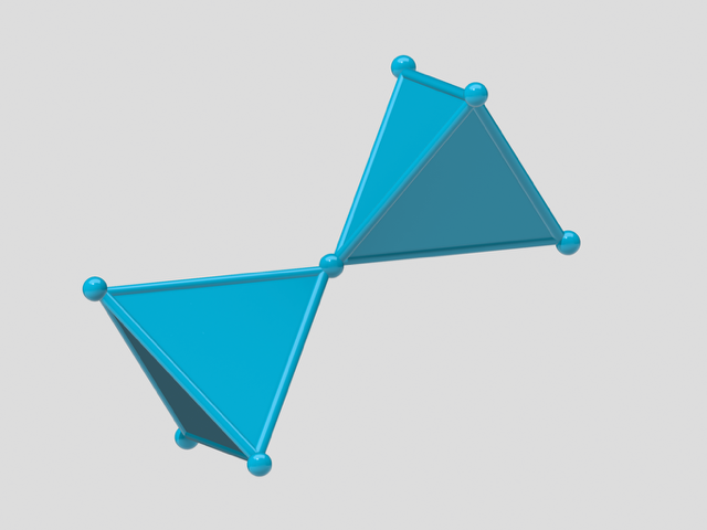
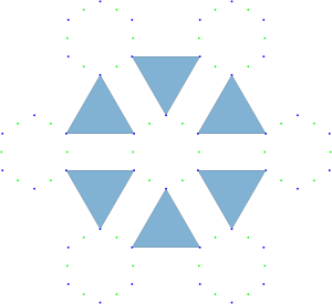
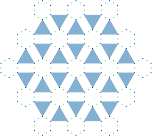
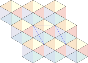
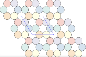
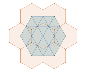
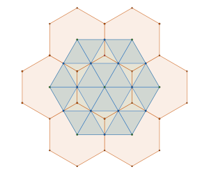
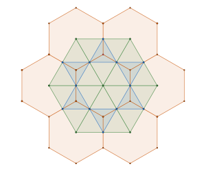
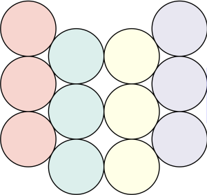
The hexagon is a radially equilateral 2-polytope. The equivalent 3-polytope is the Cuboctahedron; thus we will work with the representation of a molecule with cuboctahedral symmetry using a rigid hard sphere model (a molecule is a rigid collection of hard spheres) as visualised in the figures below.
Problem Statement
We are interested in the following question: What is the densest packing of a hard sphere molecule model with cuboctahedral symmetry?
The GEOMAG structure shown in the animation below is a good candidate. It has layers of hexagonal packings just like the perfluorobenzene structure in Chiral Interaction Energy Ground States but is it truly the densest possible configuration? I’ll leave you wondering for a bit longer (or you skip to the conclusion of the quacked case in section 6 at the end of this post).
Divide and Conquer
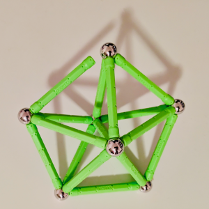
In the spirit of the divide and conquer problem solving strategy, it might be worthwhile to start with packings of simpler model molecules. Specifically, molecules having tetrahedral and octahedral symmetries like the GEOMAG constructions below, since the tetrahedron and octahedron are related to the cuboctahedron via the tetrahedral-octahedral honeycomb.
How do we know this is the optimal packing configuration of tetrahedral molecules? Well, by definition, a tetrahedral molecule is a collection of equal spheres with radius of half of the minimum distance between any two atoms of the molecule. Thus every tetrahedral molecule is a sphere packing of four spheres with equal radii. Additionally, since the kissing number of a 3-sphere is 12 (every sphere can touch a maximum of 12 neighbouring vertices) and every vertex of the GEOMAG structure belongs to exactly one tetrahedron the density of packing of tetrahedral molecules equals the Face-Center Cubic (FCC) close-packing of equal spheres, and we know we can’t get any denser packing then this due to the proof of Kepler conjecture by Thomas Hales.
The optimality of the GEOMAG octahedral molecule crystal model follows directly from the optimality of the tetrahedral variant.
From the GEOMAG constructions, we can see that there are at least two kinds of symmetries present:
1. Lattice translations – tetrahedra with the same colour are related by this isometry. The configuration of octahedral molecule models is in fact a lattice configuration. That is, the octahedral structure is generated only by a lattice group.
2. Inversions – tetrahedra and octahedra of different colours are related by this isometry. Since the regular octahedron is centrosymmetric, one can view the octahedra of different colours as inversions of each other. This introduces the inversion symmetry to the whole octahedral structure.
The lowest symmetry space group containing these isometries is the space group . See the densest packing configuration found during one optimisation run of the molecular packing algorithm’s search in the space group .
The volume of the unit cell of this structure is . Since the volume of our tetrahedral molecule is (4 times the volume of a sphere with radius ), according to the geometric packing density formula and the number of elements of factor group where is the lattice subgroup of , is , which is exactly the density of FCC close-packing of equal spheres.
Crystallographers like to assign a space group name to a structure according to its highest symmetry. The question is, what is the highest symmetry of our densest tetrahedral molecular packing? To answer this question, we have to do a quick excursion into topology, specifically “orbit-manifolds” or, for short, orbifolds.
Fibrifold Primer
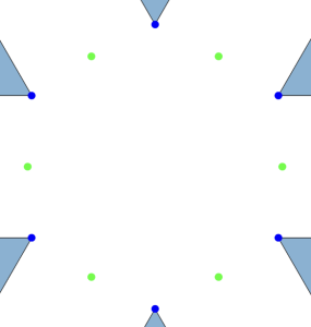
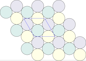
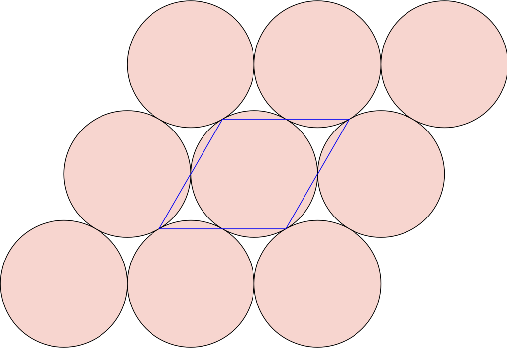
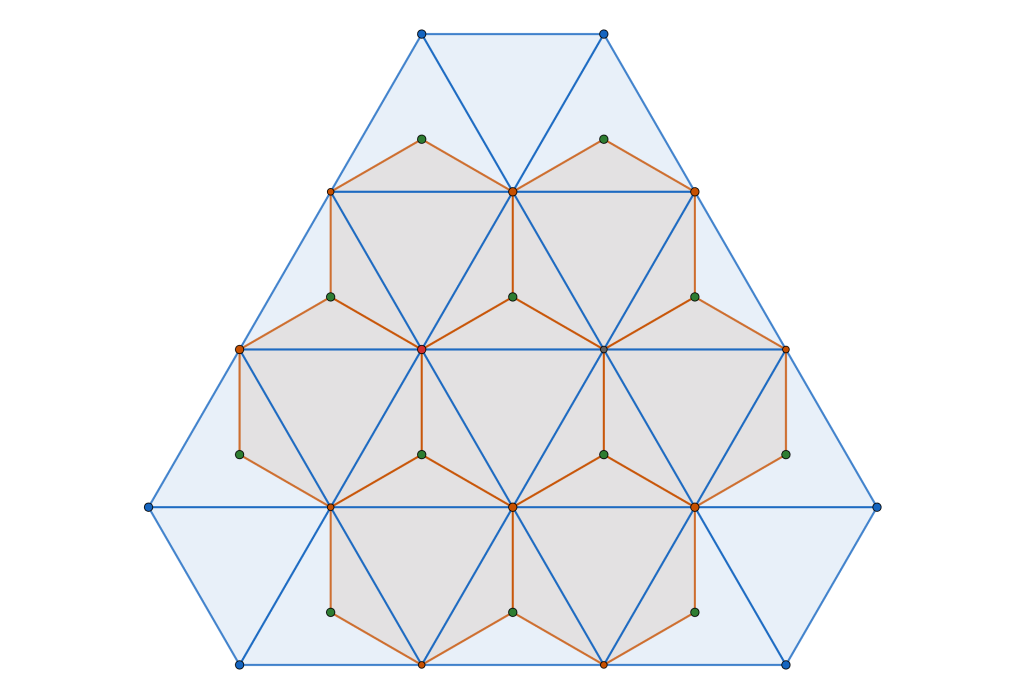
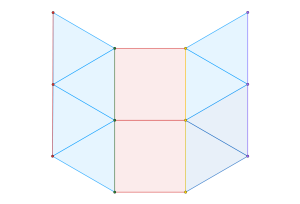
Let us take the vertices of a triangular lattice disc packing’s unit cell as highlighted by the blue parallelpiped in the image on the left below.
All four vertices are in fact centres of a 2-fold rotational symmetry as shown in the picture above on the right, making up the wallpaper group. Now if we fold up the this group by identifying the symmetry elements we end up with a surface akin to a sphere containing four singular points – points where the tangent space to the surface is not defined regularly.
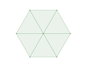
This is the orbit-manifold, for short orbifolds, representation of the crystallographic plane group . The following figure, taken from the book The Symmetries of Things by John H. Conway, Heidi Burgiel, and Chaim Goodman-Strauss, illustrates this nicely
Since we are working with space groups we need to extend wallpaper orbifolds to space groups. In essence we need to add one more lattice generator which is equivalent to multiplying (in the sense of the Cartesian product) the orbifold with a circle and thus creating a “fibered orbifold” or a fibrifold.
Geometrically a fibrifold is a fibre-bundle whose base spaces and fibres are orbifolds. In the case of space group the fibre spaces are circles . The primary fibrifold name of space group is .
Listing the Closest-Packed Symmetries
In the tetrahedral molecule packings we can notice interchanging layers of blue and red tetrahedral molecules stacked on top of each other. This is not a coincidence, these are the orbifolds of the fibrifold coupled together. There are at most three such non-isomorphic orbifold couplings in every space group. That is why some fibrifolds have a secondary or tertiary name. In the IUCr International Tables of Crystallography they are called Special Projections.
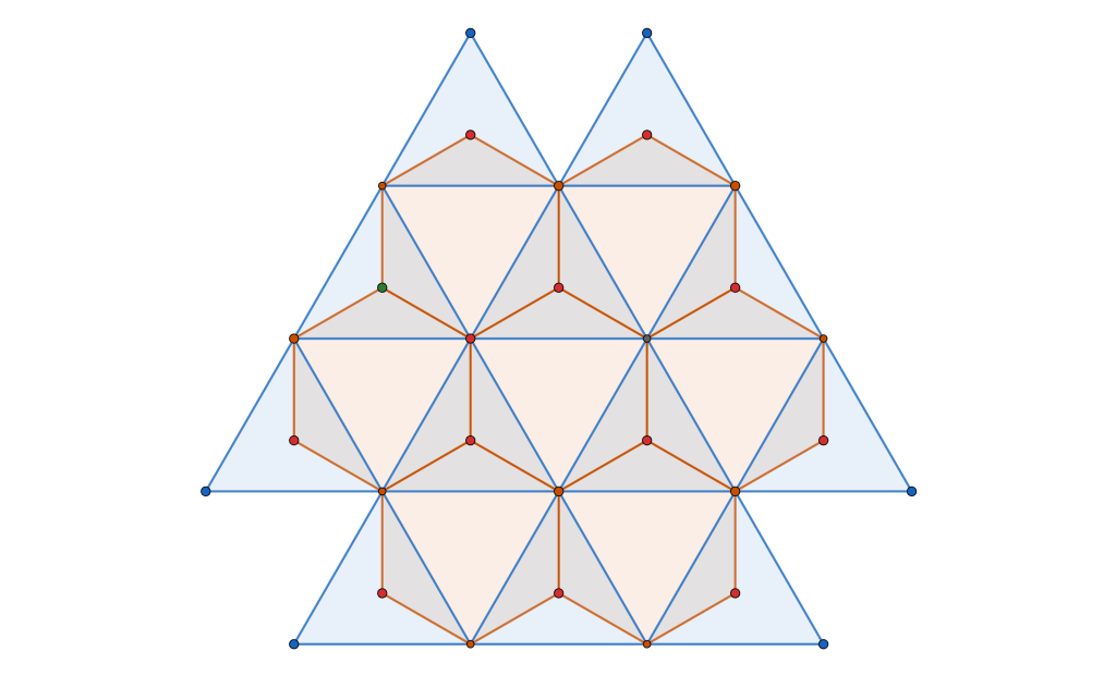
Below are these projections for the tetrahedral molecule packing.
Lattice generators of the tetrahedral molecule packing.
In this particular case the symmetries of special projections are all orbifolds i.e. the wallpaper group . These projections are reminiscent of the triangle and square tilings from our analysis of the densest plane group packings of regular convex n-gons published in Physical Review E we know that all regular n-gons attain the maximum packing density in wallpaper groups , and with orbifold names , and respectively.
|
|
|
There are only three space groups having special projections a combination of these three orbifolds. These space groups are (the space group we started with in the first place), with the fibrifold name and with the fibrifold name .
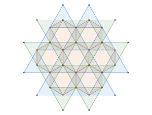
Are these the only symmetries of the tetrahedral molecular packing? No, all three special projections contain a mirror reflection. Therefore we should further our space group explorations including the wallpaper group (orbifold name ), reflected in the triangle and square tilings:
|
Thus we are adding the space groups with its fibrifold name and with its fibrifold name to our list.
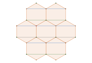
Are we done here? Not yet, one more step is necessary. Notice the (orbifold name ) square tiling symmetry in one of the tetrahedral molecular packing special projections.
|
For this reason the last space group to add to our list is . Its fibrifold name is .
All the space groups in our closest-packed list are summarised in the table below.
Navigating Singularities in Space Groups
Running searches over this space groups using our molecular packings algorithm required new a definition of an asymmetric unit in the packing algorithm for each space group such that all singular point sets of fibrifolds are contained on the boundary of the asymmetric unit. Unlike the definitions from the IUCr International Tables of Crystallography that we used before.
I wonder if companies developing software used in Crystal Structure Prediction workflows know about this unfortunate choice of asymmetric units in the IUCr International Tables of Crystallography because they also use second order numerical optimisation methods over space groups in local structure refinements and inevitably must encounter the same problem we did. Fortunately for us, equipped with the fibrifold perspective of space groups, we manage to avoid the singularities safely.
Densestand Tetrahedral Molecule Packings
For the visualisation and a brief analysis of the output configuration in the space group search, we refer to section Closest-Packed Space Groups.
As for the rest, by choosing to run searches in six very special space groups, the packing densities of all the densest molecular space group configurations with tetrahedral symmetry have the same maximal sphere packing density. The highest symmetry of the tetrahedral molecule packing in our list is . Both and have eight symmetry operations modulo lattice translations however the orthorhombic crystal system of has higher symmetry than the monoclinic crystal system of .
Densestand Octahedral Molecule Packings
Similar to the tetrahedral case, the close-packed space groups we have selected are also based on the densest octahedral molecule packing. Consequently, all densest packing configurations of octahedral molecules within these groups share the same sphere close-packing density of .
Densestand Cuboctahedral Molecule Packings
The computational experiments have confirmed our choice of symmetries for maximally dense tetrahedral and octahedral molecular packings. Therefore, the globally densest cuboctahedral molecular packing will be among the maximally dense packings in our list of closest-packed space groups.
Let’s have a look at the results from packing searches. We provide an algebraic expression for the configuration’s density alongside the numerical value in cases where we were able to determine one.
Global Cuboctahedral Molecule Packing Maximiser
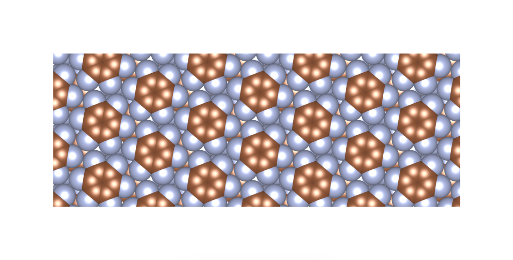
We have finally reached the conclusion of our investigation into the mystery we began with: is the GEOMAG cuboctahedral molecule packing model the global packing density maximum?
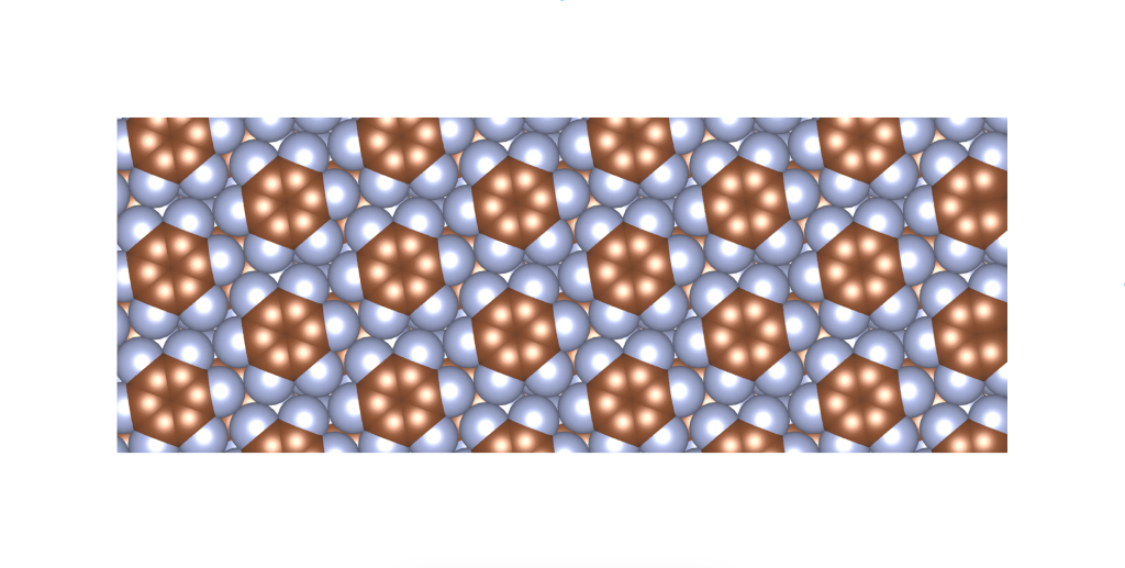
The answer is no. The structure in the animation represents the densest | packings, with a density of , which is the second densest cuboctahedral molecule packing in our list. Have a look at the comparison between the GEOMAG model and the structure from our computational experiment.
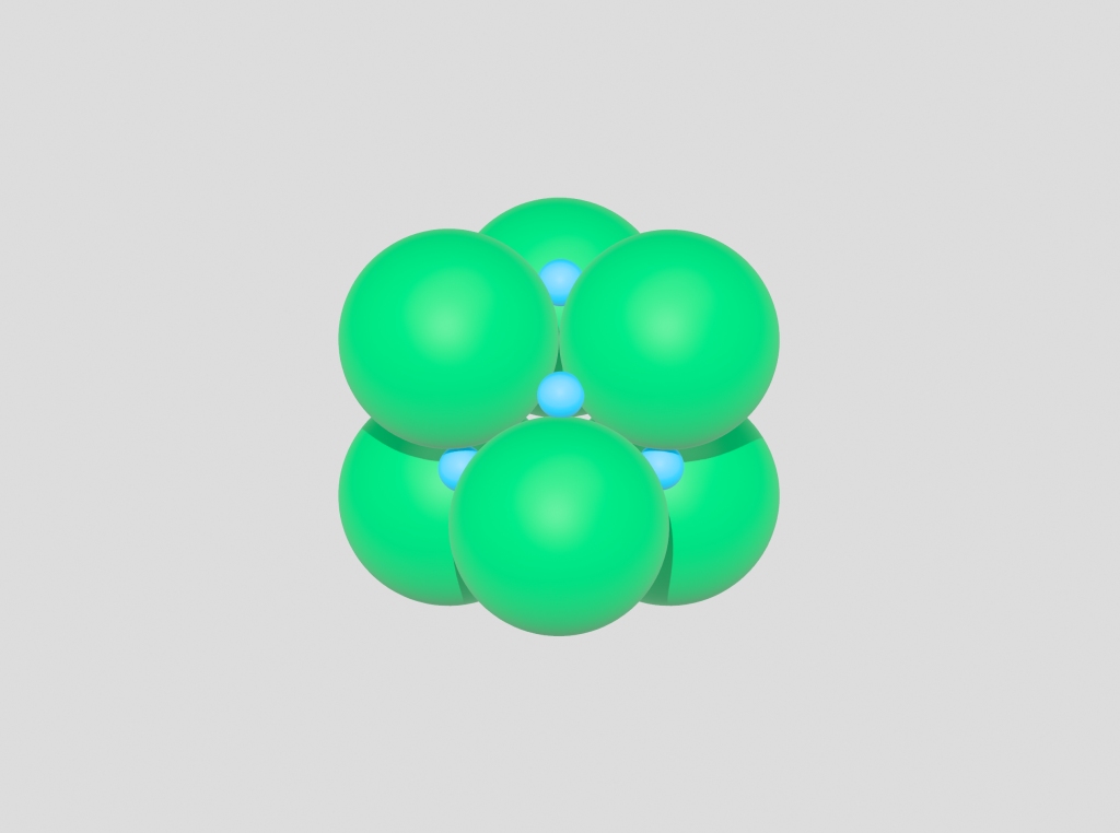
In contrast to the | configuration, the globally densest packing of cuboctahedral molecules is the configuration, which achieves a packing density of . The GEOMAG model representing this arrangement appears like this:
How do we know it is the global maximum? Well, the packing density is just short of the densest packing of equal spheres, and by construction our cuboctahedral molecule model is a collection of equal spheres with centres on the twelve vertices of a cuboctahedron, missing exactly one sphere on the inside. Conversely, the twelve spheres are in the densest possible arrangement around a single one—or shall we say—in the vector equilibrium of Buckminster Fuller.
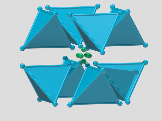
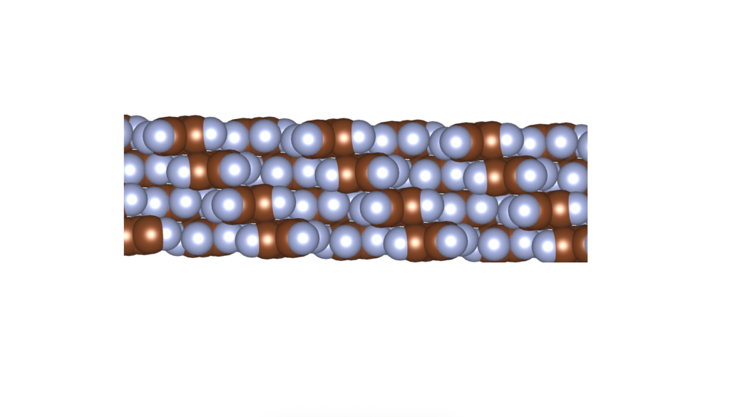
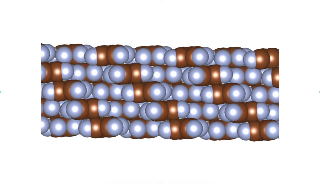
In fact, due to the radial symmetry of the cuboctahedron, the packing can be realised as a lattice packing — or, in H–M notation, as a packing — as shown in the image on the left below.
The red and green spheres represent a complementary packing to the blue cuboctahedral module packing. The spheres missing at the centre of each cuboctahedron molecule represent the centres of mass of each cuboctahedron. Moreover, the arrangement of the red central spheres in the packing lies at the vertices of a rhombic dodecahedron – an edge is created whenever any two cuboctahedra come into contact.
What is the takeaway from examining the global packing maximum configuration? We observe two levels of locally maximal close packing:
1. Atomic – Locally maximal dense packings between atoms of different molecules, where each atom touches seven atoms from neighbouring molecules.
2. Molecular – Locally maximal dense packings between molecules, where each molecule touches 14 surrounding molecules, giving each molecule a coordination number of 14.
A practical consequence of these observations is that, in our molecular packing algorithm, when searching over space groups and (both triclinic crystal systems), we need to check for overlaps up to the second neighbouring unit cells. However, when searching over space groups with the monoclinic crystal system, it suffices to check overlaps only in the first neighbouring unit cells, which speeds up packing computations substantially.
Incidentally, the rhombic dodecahedron is the cell of the rhombic dodecahedral honeycomb, which is the dual honeycomb to the tetrahedral–octahedral honeycomb with which we began our investigation. In the images below, you can see a visualisation of the rhombic dodecahedral honeycomb along a GEOMAG structure showcasing the relationship between tetrahedral, octahedral, and cuboctahedral molecular packings. Notice the inverted octet truss in the space frame generated by tetrahedral | octahedral molecular packings.
Compared to the tetrahedral and octahedral GEOMAG molecule models, the cuboctahedral molecule is not rigid. Since it is hollow on the inside (it is missing 12 bars that would otherwise stabilise the molecule model and make it rigid), it has multiple degrees of freedom of motion (see the GEOMAG Jitterbug transformation of the cuboctahedron into the icosahedron in Ionic Molecular Crystallisation Continued: Tetrahedra, Symmetry, and Salt-Like Molecular Architectures).
The interesting part of this property of the and GEOMAG models is that, in both configurations, the molecules do not collapse under the lattice forces. On the contrary, the lattice configuration structurally stabilises both models.
A direct application of this observation in materials science could be a starting point for a geometric bias to guide inverse design search for novel porous materials, for instance, using an organic molecular cage building block.
What Do the Space Groups , , , , , and Have in Common?
For one, they are relatively low-symmetry subgroups of the space group , which is the full symmetry of the face-centred cubic lattice. has 48 elements modulo lattice translations, compared with a maximum of 8 in our closest-packed space groups.
These are also the six most frequent space groups in the Cambridge Structural Database as of 1 January 2025 (CSD Space Group Statistics), accounting for approximately 82.7% of the total 1,359,039 structures. If we leave out space group , the remaining groups are all centrosymmetric, comprising 75% of the CSD in total.
The truth is, we have been somewhat misleading. Thanks to A. I. Kitaigorodsky, we had a good estimate of the closest-packed space groups from the beginning. Below is a table from the book Molecular Crystals and Molecules by A. I. Kitaigorodsky, published in 1973, showing these.
However, as a result of our cuboctahedral molecule packing explorations, we can now add an additional column to the table. To paraphrase A. I. Kitaigorodsky: for molecules with octahedral symmetry , the closest packing is attainable in space group.
Acknowledgement
I am grateful to Henry Segerman for mentioning the orbifold plane group notation during our conversation at the ICERM Geometry of Materials workshop, and for drawing my attention to the book The Symmetries of Things by John H. Conway, Heidi Burgiel, and Chaim Goodman-Strauss. From now on, I am following William Thurston’s commandment:
Thou shalt know no geometrical group save by understanding its orbifold.
In my previous post on Ionic Molecular Crystallization, I sketched a geometric analysis of a two-dimensional ionic molecular framework, guided by charged particle interactions, symmetry, and regular polygon packings. Since our real interest lies in three-dimensional frameworks, I wondered how this idea would translate into three dimensions. While still theoretical, the model feels promising—and surprisingly beautiful.
To help me visualise the constructions, I discovered a wonderful CAD modelling software, Shapr3D, which is both intuitive to use and very powerful. I had zero experience with CAD before, but within a few hours, I was able to build all kinds of three dimensional frameworks.
Let’s start with the simplest regular polyhedron—the regular tetrahedron—and build a periodic framework by connecting the vertices of tetrahedra, as shown in the picture below.
The question is: how many regular tetrahedra can share one vertex subject to crystallographic restrictions? The answer is eight, as shown in the image below. This is a simple consequence of the sphere kissing number being 12. It forms a uniform star polyhedron called an octahemioctahedron.
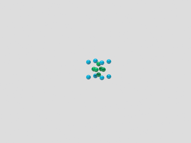
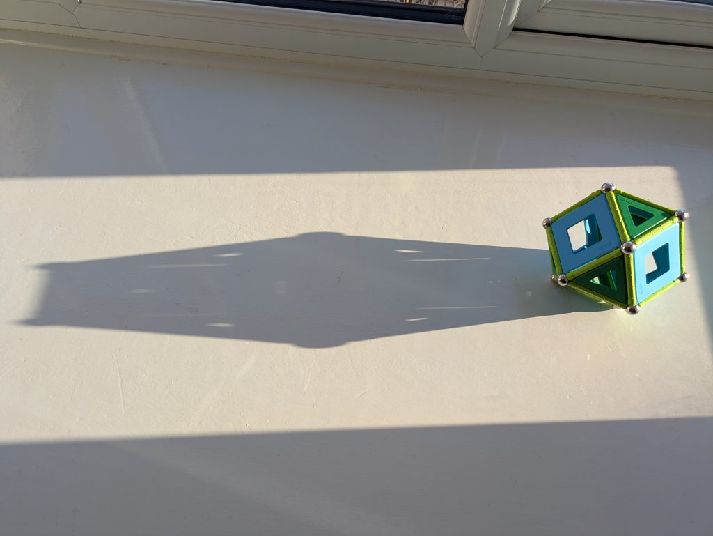
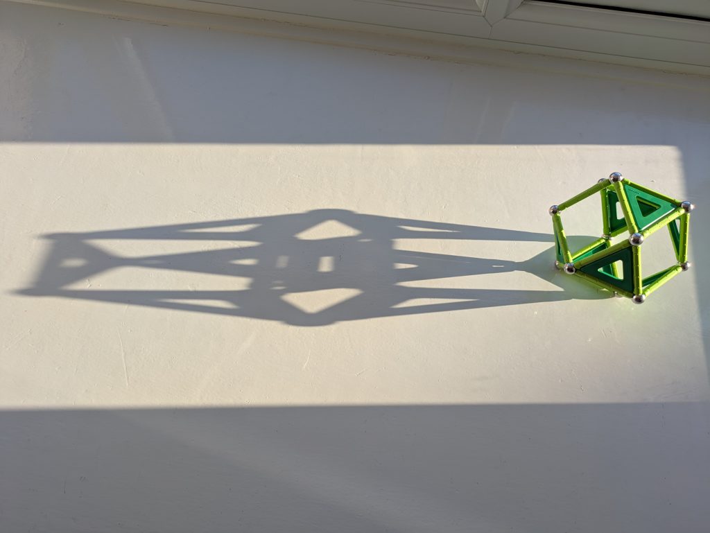
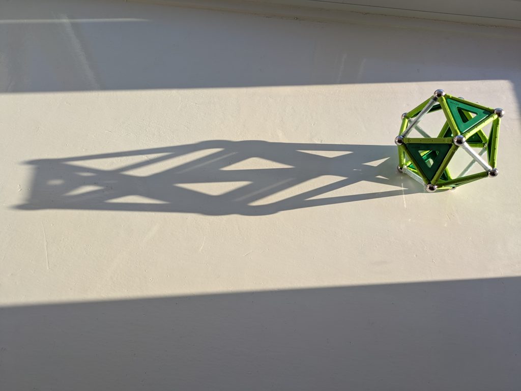
The next question is: what might a local cluster with low net electrostatic energy look like? Here is one such arrangement of blue () and green () charged particles that satisfies this criterion under the Coulomb potential.
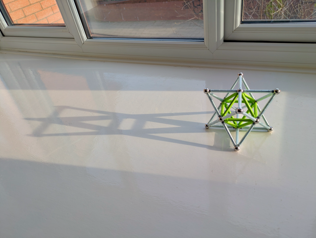
Additionally, I used the GEOMAG construction toy to build a physical model of this configuration. The green bars represent the repulsive forces in the green anion octahedral configuration. The white bars represent the attractive forces between green anions and blue cations; however, this is not entirely correct. These should not be represented as rigid rods but as tendons that can change length.
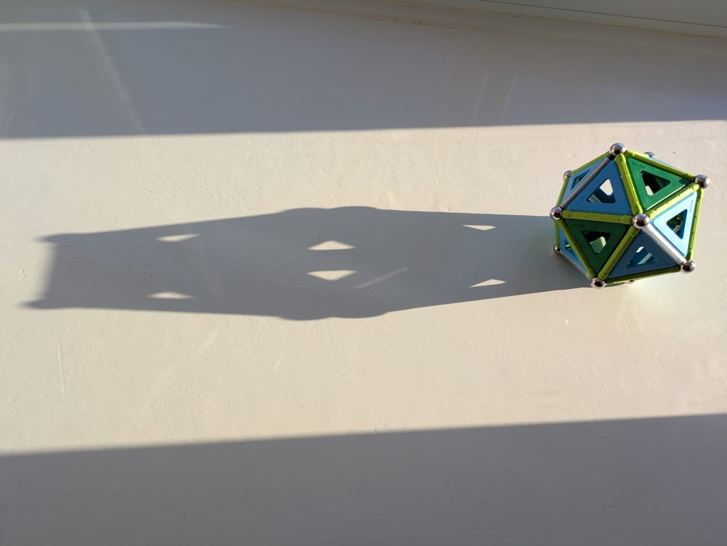
Geometrically, the GEOMAG structure represents the 1-skeleton of a stellated octahedron. The projection of the two tetrahedra, which together form the stellated octahedron, becomes visible in the shadow cast by the setting sun.
We set the configuration such that the local cluster’s Coulomb energy—introduced in the Ionic Molecular Crystallisation—is zero.
In terms of an optimisation problem, the configuration is a solution to the following:
The local configuration of positively charged tetrahedral molecules and single-atom negatively charged molecules looks like this:
Once we assemble these octahemioctahedra, the resulting framework exhibits symmetry (space group 225)—the same as fluorite (). The similarity is not merely mathematical; chemically, the tetrahedral framework model could approximate a real organic fluorite structure, provided we can identify the appropriate molecular analogue.
One can view this as the tetrahedral-octahedral honeycomb, where the octahedral building blocks have been removed. I positioned the camera to highlight the six-fold and four-fold roto-inversions of the framework.
Following the two-dimensional triangular tiling case, I constructed the following framework by removing tetrahedra from the framework while preserving crystallographic symmetry:
This is the three-dimensional equivalent of the lowest-density triangular configuration (Kagome lattice) from the Ionic Molecular Crystallisation post—the quarter cubic honeycomb. Its space group is (space group 227), same as diamond, and it is mechanically quite stable, as shown in the photo below.
A view of the diamond-like tetrahedral framework (via Shapr3D’s augmented reality feature) placed next to Henry Segerman’s 3D printed model of an auxetic mechanism at the ICERM Geometry of Materials workshop. Both models have the same symmetry.
As in the case of triangular tiling, there is a group-subgroup relationship between the tetrahedral-octahedral and the quarter cubic honeycombs via the space group (space group 224). is the maximal index -subgroup of , and is the maximal index -subgroup of . This should not come as a surprise given how the framework was constructed.
If the observations from the two-dimensional framework analysis translate to three dimensions, this framework should represent a local Coulomb energy minimum, and a global minimum if the symmetries of the molecular system are constrained to the space group symmetry isomorphism class.
Similar to triangular frameworks, one can associate a sphere packing with the tetrahedral framework, and further with a regular -polytope, using these to enumerate local energy minima.
This suggests a potential geometric design principle: Higher symmetry often corresponds to greater mechanical stability, whereas its sub-frameworks may offer larger pores or other advantageous properties at the expense of rigidity.
In other words, if our Coulomb cluster-tetrahedral structure minimises energy under symmetry, then the lower-symmetry frameworks derived from it (e.g., ) may also represent local minima—stable enough to exist, but metastable within the full energy landscape.
Moreover, we can define a generative method for exploring neighbourhoods of local energy optima by sampling an entire family of ionic molecular frameworks through the simple identification of symmetry-breaking subgroups of a highly symmetrical parent structure. That is, we begin with the framework exhibiting the highest symmetry and then systematically investigate its symmetry-reduced subframeworks.
Interestingly, some coarse-grained molecular simulations already approximate molecules as rigid polyhedra. Our goal is to create stable framework models with large cavities, which may serve as blueprints for the computational design of organic frameworks, applicable to areas such as atmospheric water harvesting and CO₂ capture.
and the following absolutely symmetric quadratic form:
courtesy of K. L. Fields (K. L. Fields, 1979. Stable, fragile, and absolutely symmetric quadratic forms. Mathematika, 26(1), 76–79).
This brings us full circle to the symmetries of FCC sphere packing explored in these blog posts:
Based on these, A. I. Kitaigorodsky (link to German Wikipedia page as no English version exists) formulated his Close Packing Principle:
“The mutual arrangement of the molecules in a crystal is always such that the ‘projections’ of one molecule fit into the ‘hollows’ of adjacent molecules.”
— From Molecular Crystals and Molecules by A. I. Kitaigorodsky
So, what’s next? I’m now looking into how kinematics of the cuboctahedron under space group symmetry constraints can help identify which polyhedral frameworks are mechanically stable—and which ones are just aesthetically pleasing. After my visit to ICERM and a conversation with Robert Connelly, I’m convinced that the mathematics of tensegrities is the key.
From left to right: Transformation of a cuboctahedron into an icosahedron through the continuous motion of the triangular faces of the cuboctahedron. As in the stellated octahedron GEOMAG model, the white edges should not be rigid but elastic.
During her visit to Liverpool, Zuzka—my fiancée Lina’s mom—gifted us these glass geodesic polyhedra. When sunlight shines through them, it scatters across our living room walls, creating miniature rainbows.
This is, in fact, the basic idea behind X-ray diffraction, discovered by Max von Laue in 1912. When electromagnetic waves-such as X-rays-pass through a crystal, the symmetrical arrangement of atoms causes the waves to diffract. When these waves hit an impenetrable surface, we can photograph the resulting wave interference pattern, composed of both constructive and destructive interactions.
One key challenge in X-ray crystallography is reconstructing a crystal’s atomic structure from its diffraction pattern—an example of an inverse problem. For instance, the mini-rainbow triangular lattice in the photo arises from the six-fold rotational symmetry of our two glass tetrahedral geodesic polyhedra.
The idea of hanging transparent geodesic shapes in front of the window—creating rainbows across the room—came from Lina’s dad and my teacher, Oleg Šuk. He experimented with different materials, including an acrylic geodesic heart (with “acrylic” referring here to PMMA photonic crystal). I can’t help but wonder if the Šuk family is secretly guiding my work. See my previous posts, Chiral Interaction Energy Ground States and Yayoi Kusama’s Chandelier of Grief: Symmetry in Art and Science, for additional context.
A few months ago, I encountered an interesting problem related to molecular crystallization. Consider a two-dimensional system with two types of molecules: the first type consists of rigid triangles with positive charges localized at the vertices (shown as blue triangles in the image below), and the second type is a single-atom molecule with a negative charge (shown as a green dot).
Our key questions are:
Does this molecular system crystallize in the thermodynamic limit?
If so, what are the characteristics of its ground states?
Let’s assume the system’s intermolecular interactions follow a normalized Coulomb/electrostatic potential:
where and denote molecules of either type (green negative or blue positive triangular), is the Euclidean distance between charges and . For green particles, , while for vertices of blue triangles, . This creates attractive forces between opposite charges and repulsive forces between like charges, proportional to their relative distance.
The intermolecular energy is defined as the sum of all pairwise interactions between molecules and :
This quantity generally lacks an infimum, so we need additional constraints.
We aim to find a sequence of molecular configurations where the following limit converges to a constant:
Here, represents a collection of molecules of both types ().
Let’s focus on local clusters, as shown below:
For any where , an alternating configuration of charges in a local cluster can found for any . Moreover, due to the rigidity of triangular molecules and the form of the potential , the maximal cluster contains charges.
In our example cluster, , we set the energy to:
for demonstration purposes.
Alternatively, the cluster configuration can be expressed in the form of the optimization problem:
In the configuration, the blue positive charges occupy the interstitial voids of the hexagonal close-packed arrangement of negative green charges:
Following these local optimizations, we define a quantity we call the energy per cluster as:
where is an index set . Minimizing for such a cluster collection becomes a well-defined problem:
For cardinality , the solution is illustrated below.
Note that the interaction potential respects molecular memberships—for and , we require .
We can expand to :
or any .
What we did is that we transformed the problem of finding molecular system minimizers into finding minimizers of a single-particle system with potential for , and we already know that the global minimizer is a dilated, translated, or rotated version of the triangular lattice.
Geometrically, this transformation effectively contracts local clusters into single points, resulting in a regular triangular tiling:
Having resolved the crystallization question, let’s examine the ground states’ characteristics, starting with a natural question: Are there other possible crystal phases? (From the materials science perspective, this question is important because of Crystal polymorphism)
On one side we can view our ground state configuration as a triangular tiling because of the rigidity of the blue molecules. On the other side, because of the way we have reframed the intermolecular interactions in terms of pairwise cluster interactions we may view the ground state configuration as the triangular lattice. The connecting point of these two views are the Archimedean circle packings and their associated semi-regular tessellations.
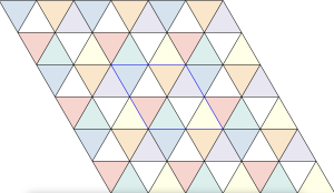
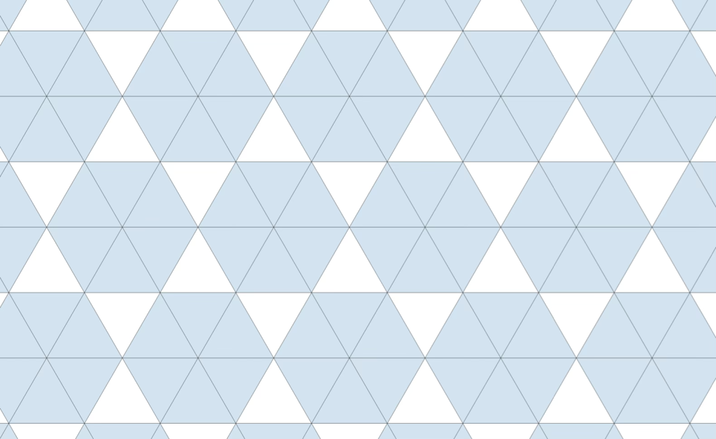
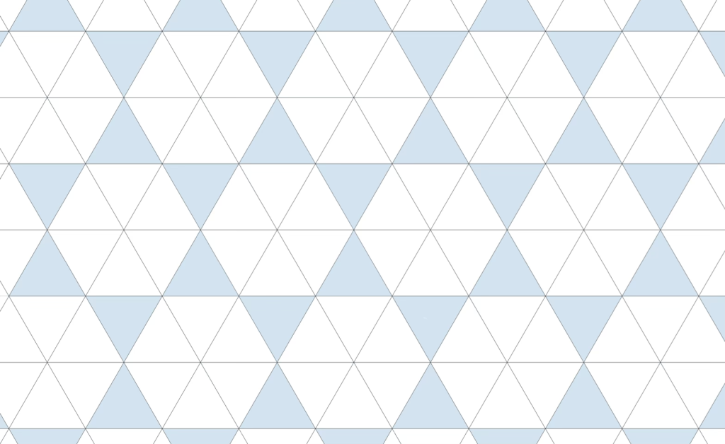
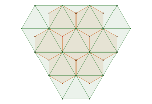
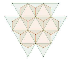
The densest packing of regular triangles is the configuration with a density of . It is, in fact, a tiling of triangles as shown below.
The maximal non-isomorphic subgroup of is the plane group. The densest packing of regular triangles when the packing configurations are restricted to the isomorphism class has a density of and is shown in the image below.
This is, in fact, a consequence of removing one of the mirror symmetries from the plane group.
Another way to get here is to look at , the Archimedean framework
associated with the disc packing with packing density of
, and the Archimedean framework associated with the hexagonal close packed configuration of disc with density
and its associated Archimedean framework
By interlacing the hexagonal and triangular frameworks
we construct new framework. The common (blue) intersection point of the hexagona and triangular frameworks in fact define a triangular sub-tiling
and the p is constructed by removing triangle tiles containing a vertex at its center of mass
Alternatively we can create a complementary triangle packing with density of by removing tiles not containing an interior vertex
The resulting structure is sometimes referred to as the Kagome Lattice, although it is not a lattice per se.
Starting from the triangle packing which is in fact a tiling
and decomposing it into two complementary packings with symmetry with density of
This should come as no surprise since is the a maximal t-subgroup of of index 3.
To demonstrate this point, we start again from the disc packing framework
and interlace it with the triangular framework associated with packing of discs
in such a way that disc centers are are subsets of the hexagon vertices
and we remove one symmetry from the tiling, the one not having a hexagon vertex at its center.
In fact, there are two possibilities to achieve the same result by using the triangle tiling above and rotating it by with respect to zero (center of the middle pentagon).
and do exactly the same thing as previously to get the second triangle tiling
Combining these two triangle packings,
the symmetry of should be clearly visible.
This tiling is a isomorphic to the one of the Archimedean (semi-regular vertex transitive) tilings associated with the densest packing of discs with density of
with it’s semi-regular tiling
These constructions are nothing new. For a comprehensive treatment of regular and semi-regular tilings, I recommend Regular Polytopes by H. S. M. Coxeter, first published in 1947. (Coxeter was the geometer who inspired M. C. Escher, which resulted in the Circle Limit I–IV series.)
Returning to our original problem of characterizing and enumerating possible Coulomb potential ground states of our molecular system, all these triangle packings represent viable local energy minima. This conclusion follows from our transformation of the intermolecular interactions into a nearly spherically symmetric “energy per cluster” potential, which preserves all symmetries of the hexagonal close-packing configuration of discs: p2, p2gg, pg, p3, and p1, as well as the rigidity of the triangular molecule.
We have classified the packings by associating each configuration with Archimedean disc packings and tessellations. The global energy minimizer corresponds to the triangular tiling and lattice, as demonstrated by Theil in “A Proof of Crystallization in Two Dimensions” (Commun. Math. Phys. 262, 209–236, 2006). https://doi.org/10.1007/s00220-005-1458-7. Since all our configurations are subsets of the triangular tessellation relative to some tiling symmetry subgroup, they are energy minimizers within their respective symmetry groups. (See Bétermin, L. “Effect of Periodic Arrays of Defects on Lattice Energy Minimizers,” Ann. Henri Poincaré 22, 2995–3023, 2021. https://doi.org/10.1007/s00023-021-01045-0.)
A property of Archimedean tessellations is that they are vertex-transitive, meaning the same number, , of regular -gons meet at each vertex. In triangular tessellations, six regular triangles (-gons) meet at each vertex. For regular tessellations like the triangular one, this follows a simple equation:
This is only for one type of polygon, but we have more types. However, we can generalize this formula to n-types of polygons:
For example, the tessellation associated with the packing of discs shown above has every vertex surrounded by regular -gons (triangles) and regular -gons (squares).
Ultimately, the equation above is simply a disguised form of the Euler characteristic for plane-connected graphs induced by the vertex figure of a semi-regular tessellation.
What does this mean in the context of our molecular system?
The vertex figure of each ground state is determined by the leading contributions to its total energy.
Combined with the Crystallographic restriction theorem, this formula allows us to explore possible ground state configurations based on molecular shape. In a periodic configuration, for every , there exists at least one such that the expression holds. Thus, for any such -gon shaped molecule, the vertex figure equation has only a finite number of integer solutions. Unfortunately, in cases like the pentagon, we might need to delve into the realm of aperiodic tilings.
Additional Notes
In this blog, we considered the existence and structure of the minimisers of a simple Coulomb electrostatic energy in the context of a model two-dimensional ionic molecular system.
Conversely, if we assume that the ground state of this ionic molecular system corresponds to the configuration of the 19 ionic clusters shown previously, then, as tends to infinity, the energy per cluster, , is essentially an instance of the Madelung constant, up to a scaling constant.
Furthermore, the local cluster configuration defines a configuration polygon and the solutions of for and correspond to ground states of the configurational energy constrained by a constant average concentration. For more details, see Sanchez, J. M., & De Fontaine, D. (1981).Theoretical Prediction of Ordered Superstructures in Metallic Alloys.in O’Keeffe, M. & Navrotsky, A. (Eds.). Structure and Bonding in Crystals Volume II, 2, 117-132.
Moreover, the treatment of ionic crystals using the interstitial voids of eutactic structures, as detailed in the book Crystal Structures: Patterns and Symmetry by Michael O’Keeffe and Bruce G. Hyde (first published in 1996 by the Mineralogical Society of America and recently reprinted by Dover Publications), provides additional context for our ionic molecular crystal model. In a sense, the instance considered here can be regarded as an extension of the description of monoatomic ionic compounds to ionic molecular systems.
Additionally, Madelung energy, a quantity related to Madelung constants and recently applied in the context of organic salts by Izgorodina, E. I., Bernard, U. L., Dean, P. M., Pringle, J. M., and MacFarlane, D. R. (2009) in The Madelung Constant of Organic Salts, Crystal Growth & Design, 9(11), 4834–4839, is somewhat reminiscent of our ionic molecular crystal model.
A few days ago, my beloved fiancé surprised me with a GEOMAG construction toy for my birthday. GEOMAG consists of small rods with embedded magnets and metallic spheres that can be assembled into various structures. It’s truly amazing—I had no idea something like this existed!
It can also demonstrate structural rigidity problems, as shown in this framework
which becomes flexible after removing just one link.
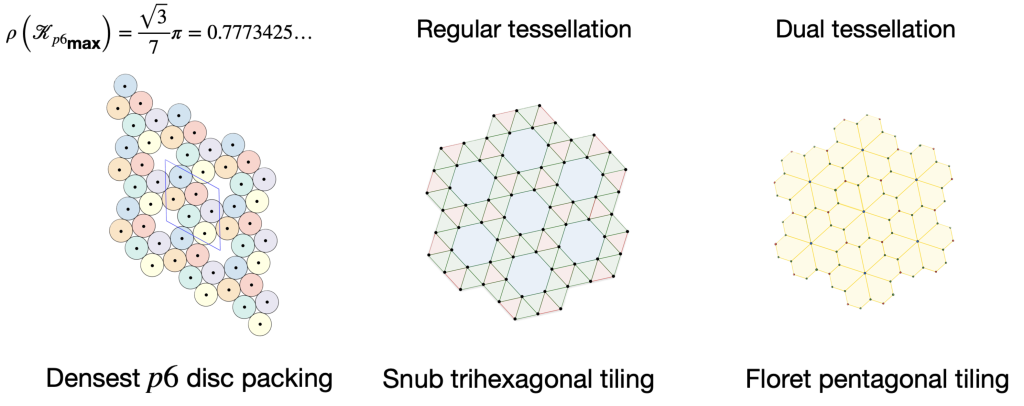
The stable framework is actually the snub trihexagonal tiling – a regular tessellation associated with the p6 packing of discs.
This framework is created by drawing links between the centers of touching disks. The tessellation on the right is called a floret pentagonal tiling. We can create this tiling from the
p6 packing of hexagons
by connecting each hexagon’s edge vertices to their nearest lattice points.
From the crystallographic perspective, the vertices of the dual tessellation lie in the
interstitial sites of the regular tessellation. Thus, the circles of the p6 packing are incircles of the pentagons in the floret pentagonal tiling and the hexagons in the hexagonal p6 packing.
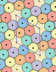
This serves as a physical model of the Lennard-Jones system I described in my blog entry Lennard-Jones hexagonal molecular system. Through this model, I discovered that there are two chiral ground states connected by a continuous path in the configuration space.
Take a look at the animation below to see how it all works!
This is closely related to the vibrational part of lattice energy, degrees of freedom and structural stability of molecular crystals. Let’s have closer looks at this.
Below is a visualization illustrating the transition between the chiral ground states of a 3-molecule cluster. Each molecule in the cluster contains six atoms. The intermolecular energy is given by the Lennard-Jones potential:
where is the Euclidean distance between the -th atom of molecule and the -th atom of molecule , as shown in the image below.
The chiral ground states are in clear energy potential wells and represent two different global solutions of the energy cluster minimization problem.
From the GEOMAG model animation, one can imagine this cluster being held together only by the forces between nearest neighbors. By relaxing three of the total interactions, one introduces a single degree of freedom into the otherwise rigid cluster, allowing the configuration to shift into its neighbouring potential well.
However, this requires an interaction potential that decays to zero sufficiently quickly as the distance approaches infinity, since pairwise interactions among all atoms of different molecules are included, not only the first neighbours. The Lennard-Jones potential is one such example, where the leading contribution to the overall energy comes from the three-atom cluster in the middle, and the transition from one ground state to the other is animated as revolving around the centre of mass of this cluster.
It is also by this Lennard-Jones potential property that the ground state of this two-dimensional molecular system coincides with the densest packing of discs. This means that there are also two chiral densest packings of all -gons with six-fold rotational symmetry. This observation connects directly to my earlier work on plane group packings during my PhD, as it shows an aspect these packings I overlooked. The results of this study are published in our Densest plane group packings of regular polygons manuscript.
Moreover, this explains the crystal defects in the Lennard-Jones hexagonal molecular system. Since mirror symmetry is not permitted in this two-dimensional system, we observe incompatible local ground state patches.
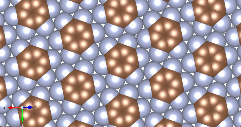
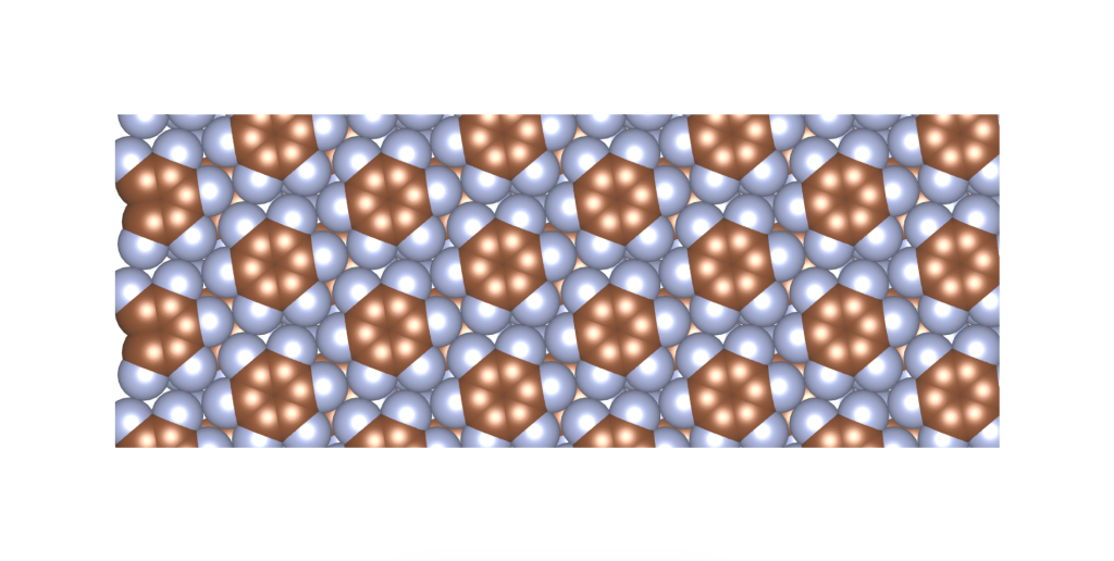
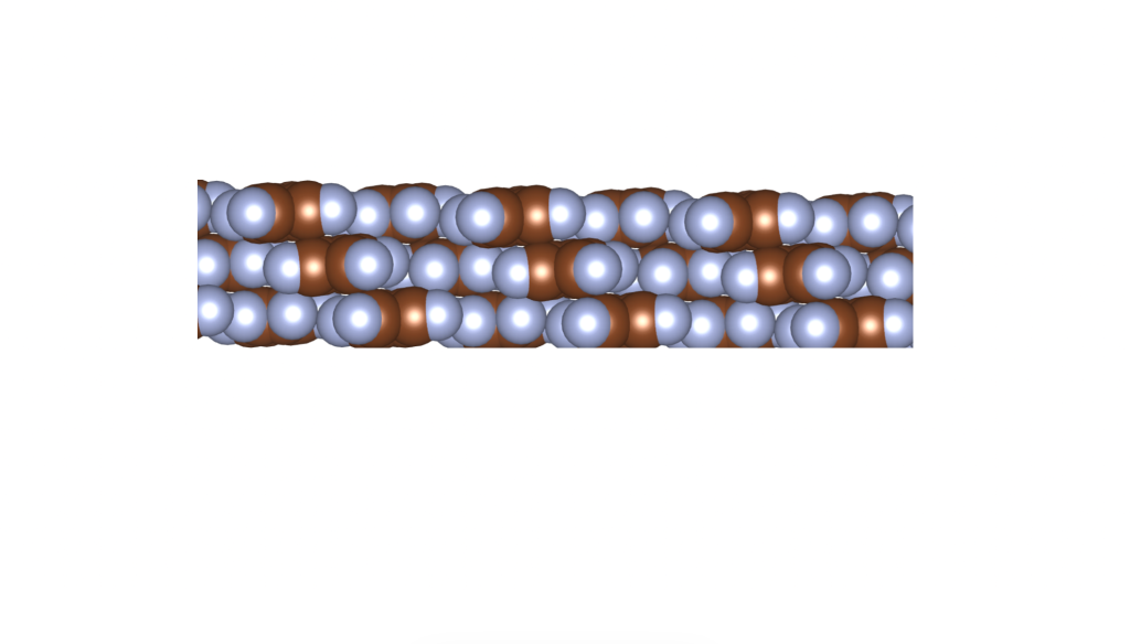
I was wondering if a real material with this crystal structure exists. In fact, it does, and it was published only a few years ago. See the image and reference below.
Rusek, M., Kwaśna, K., Budzianowski, A., & Katrusiak, A. (2019). Fluorine··· fluorine interactions in a high-pressure layered phase of perfluorobenzene. The Journal of Physical Chemistry C, 124(1), 99-106.
The above is a space-filling visualization of this high-pressure phase of perfluorobenzene, which is in excellent agreement with our highly simplified model. The sphere radii are set to the van der Waals radii. The left image shows one layer, while the right image displays the same layer with the carbons removed. The space group of this crystal is C2/c. C2/c symmetry consists of a two-fold rotational symmetry (here, within one layer of perfluorobenzene) and a perpendicular mirror symmetry. This effectively means that the layers alternate as two chiral two-dimensional ground states, interchanging chirality layer by layer.
S – enantiomer
R – enantiomer
S – enantiomer
Why is this important beyond just creating appealing pictures and animations? One reason is that it can significantly reduce computational time complexity by eliminating unnecessary calculations in
Crystal Structure Prediction (CSP). For example, if we know beforehand that our target compound satisfies a few assumptions, the degrees of freedom to explore can be reduced to a maximum of 12, sometimes even less, as demonstrated in our Close-Packing approach to CSP (Alternatively, we can think of the hard sphere model as a pairwise interaction potential. However, in this blog, we are considering soft core interactions).
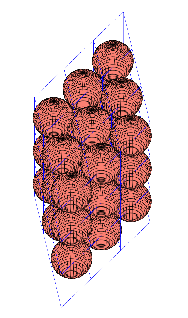
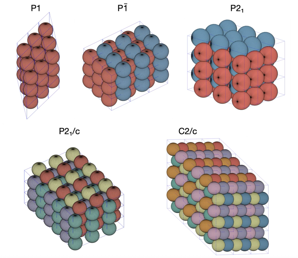
In this post, we’re diving back into the world of sphere packings, focusing on the space groups and . Feel free to check out an earlier discussion on Densest P1, P-1 and P21/c packings of spheres. Both of these groups reach the packing density of .
The densest packing almost identical to the group. Even though they belong to different crystal systems—triclinic for and monoclinic for —they share the same unit cell parameters: , , and . Here’s a snapshot of what this packing looks like:
Next up is the space group, which also falls under the monoclinic category. This group is a bit more complex, with eight symmetry operations. Its densest packing has unit cell parameters of , , and . Check out the illustration below of the densest packing configuration:
So far, we’ve seen that the optimal packing density for the space groups , , , , and matches the general optimal sphere packing density. This isn’t too surprising since these groups are all related to the Hexagonal Closed Packed structure, via group – subgroup relations. Interestingly, these space groups are among the top ten of the most frequently occurring in the Cambridge Structural Database, making up 74% of its entries.
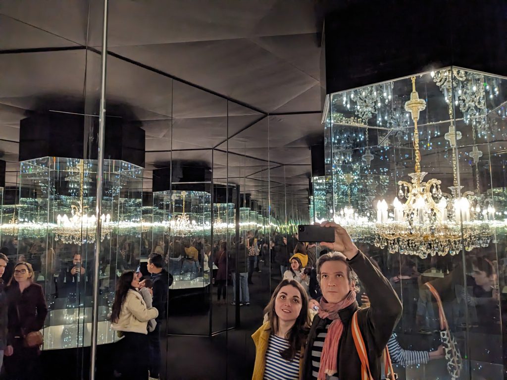
This photo captures my fiancé Lina and myself at Yayoi Kusama’s “Infinity Mirror Rooms” exhibit at Tate Modern in London, taken in March 2024. The installation, called “Chandelier of Grief,” uses mirrors and light to explore ideas about symmetry.
The centrepiece of the artwork is a chandelier surrounded by six mirrors arranged in a regular hexagonal prism. This creates an interesting visual effect—an infinite lattice of chandeliers extending in all directions, with each reflected chandelier appearing at the centre of symmetry within this lattice.
What we’re experiencing is a visual representation of a hexagonal lattice, one of the five two-dimensional Bravais lattices. Mathematically, it represents a discrete group of isometries in two-dimensional Euclidean space. The point group of this hexagonal lattice is isomorphic to the dihedral group , highlighting its sixfold rotational symmetry and mirror reflection properties.
Physically, the hexagonal lattice emerges as the ground state configuration for systems of particles interacting via certain potentials, such as the Lennard-Jones potential, in the thermodynamic limit. Moreover, the hexagonal lattice is realised in materials like graphene, where carbon atoms arrange themselves in this highly symmetric pattern, leading to its unique properties.
Kusama’s installation is not only aesthetically pleasing but also serves as a visual representation of abstract concepts in mathematics and physics. The infinite reflections illustrate how artistic expression can intersect with scientific principles, making complex ideas accessible and engaging to a wider audience.
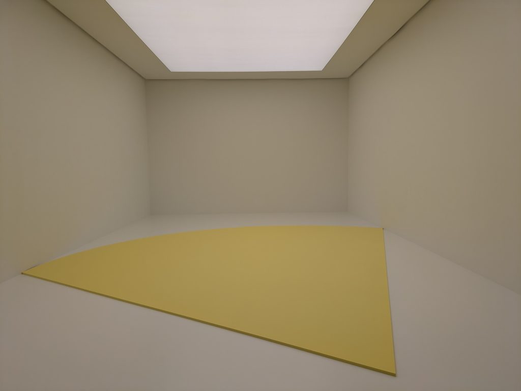
 Cuboctahedral Molecule Packing configuration from the Densest Packings of Cuboctahedral Molecules post.
 framework of Claude Code CLI.


 . See the densest packing configuration found during one optimisation run of the molecular packing algorithm’s search in the space group


 . Since the volume of our tetrahedral molecule is
  (4 times the volume of a sphere with radius
  ), according to the geometric packing density formula
  and the number of elements of factor group
  where
where  is the lattice subgroup of
  , is
, is  ,
,  which is exactly the density of FCC close-packing of equal spheres.


 wallpaper group. Now if we fold up the this group by identifying the symmetry elements we end up with a surface akin to a sphere containing four
 orbifold with a circle and thus creating a “fibered orbifold” or a
  . The primary fibrifold name of space group
  .
.


 and
and  with orbifold names
  and
and  respectively.


 with the fibrifold name
  and
and  .
.
 (orbifold name
  ), reflected in the

 with its fibrifold name
  and
and  with its fibrifold name
  to our list.
 (orbifold name
  ) square tiling symmetry in one of the tetrahedral molecular packing special projections.


 . Its fibrifold name is
  .
.
![\[ \begin{tabular}{ll|ll|ll|ll} \hline \hline \multicolumn{8}{c}{\textbf{Symmetries of the} $\mathbf{P\bar{1}}$ \textbf{Tetrahedral and Octahedral Molecule Packings}} \\ \hline \multicolumn{2}{c|}{\textbf{Closest-Packed Space Groups}} & \multicolumn{6}{c}{\textbf{Symmetries of Special Projections}} \\ \hline \textit{H-M} & \textit{Fibrifold (primary)} & \textit{H-M} & \textit{Orbifold} & \textit{H-M} & \textit{Orbifold} & \textit{H-M} & \textit{Orbifold} \\ \hline $P\overline{1}$ & (2 2 2 2) & $p2$ & 2 2 2 2 & $p2$ & 2 2 2 2 & $p2$ & 2 2 2 2 \\ $P2_{1}$ & ($2_{1} 2_{1} 2_{1} 2_{1}$) & $pg$ & $\times \times$ & $pg$ & $\times \times$ & $p2$ & 2 2 2 2 \\ $P2_{1}/c$ & ($2_{1} 2_{1} 2 2$) & $p2mg$ & 2 2 * & $p2gg$ & 2 2 $\times$ & $p2$ & 2 2 2 2 \\ $C2/c$ & ($2_{0} 2_{1} 2 2$) & $c2mm$ & 2*2 2 & $p2mg$ & 2 2 * & $p2$ & 2 2 2 2 \\ $P2_{1}2_{1}2_{1}$ & ($2_{1} 2_{1} \overline{2}$) & $p2gg$ & 2 2 $\times$ & $p2gg$ & 2 2 $\times$ & $p2gg$ & 2 2 $\times$ \\ $Pbca$ & ($2_{1} 2\overline{*} :$) & $p2mg$ & 2 2 * & $p2mg$ & 2 2 * & $p2mg$ & 2 2 * \\ \hline \end{tabular} \]](https://milotorda.net/wp-content/ql-cache/quicklatex.com-7feaf7092df8b1622f700599e7a496b2_l3.png "Rendered by QuickLaTeX.com")
 and
and  Tetrahedral Molecule Packings
 and
and 


 .
.


 and
and 


 , which is the second densest cuboctahedral molecule packing in our list. Have a look at the comparison between the GEOMAG model and the structure from our computational experiment.


 . The GEOMAG model representing this arrangement appears like this:


 short of the densest packing of equal spheres, and by construction our cuboctahedral molecule model is a collection of equal spheres with centres on the twelve vertices of a cuboctahedron, missing exactly one sphere on the inside. Conversely, the twelve spheres are in the densest possible arrangement around a single one—or shall we say—in the vector equilibrium of
  packing — as shown in the image on the left below.


 ,
,  ,
,  ,
,  ,
,  , and
, and  , which is the full symmetry of the face-centred cubic lattice.
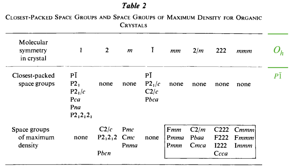

 . See
. See 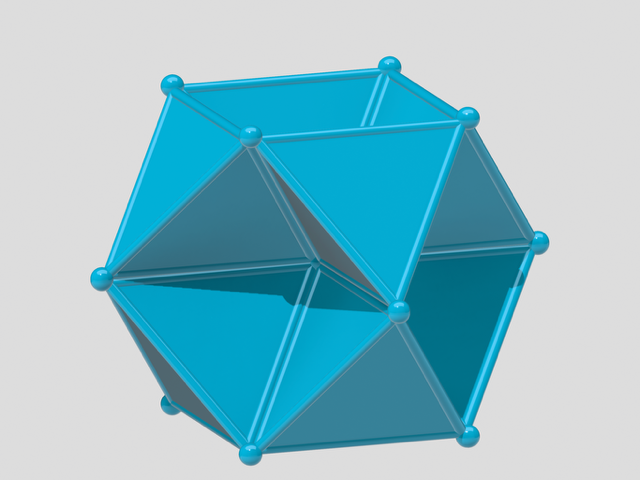
 ) and green (
 ) charged particles that satisfies this criterion under the Coulomb potential.

![\begin{equation*} C_0 = \text{argmin}_{\iota:C_0 \rightarrow \mathbb{R}^{2k}} \left[ E^{C}(C_0^{\iota}) \right]^2 \end{equation*}](https://milotorda.net/wp-content/ql-cache/quicklatex.com-fbe580ac2647632148f2224fd5efe19d_l3.png "Rendered by QuickLaTeX.com")
 ). The similarity is not merely mathematical; chemically, the tetrahedral framework model could approximate a real organic
 (space group 227), same as diamond, and it is mechanically quite stable, as shown in the photo below.

 (space group 224).
 -subgroup of


 and
and  denote molecules of either type (green negative or blue positive triangular),
  is the Euclidean distance between charges
  and
and  . For green particles,
  , while for vertices of blue triangles,
  . This creates attractive forces between opposite charges and repulsive forces between like charges, proportional to their relative distance.
 between molecules
 where the following limit converges to a constant:

 represents a collection of
  molecules of both types (
 ).
).
 , an alternating configuration of charges in a local cluster can found for any
  . Moreover, due to the rigidity of triangular molecules and the form of the potential
  , the maximal cluster contains
  charges.
 , we set the energy to:

![\begin{equation*} C_0 = \text{argmin}_{\iota:C_0 \rightarrow \mathbb{R}^{2k}} \left[ E^{C}(C_0^{\iota}) +1 \right]^2 \end{equation}](https://milotorda.net/wp-content/ql-cache/quicklatex.com-3e7577ae5bfe3cd94d7847e44f750a29_l3.png "Rendered by QuickLaTeX.com")
 configuration, the blue positive charges occupy the
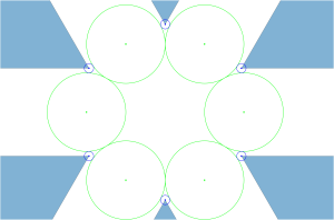

 is an index set . Minimizing
  for such a cluster collection becomes a well-defined problem:

 , the solution is illustrated below.
 respects molecular memberships—for
  and
and  , we require
  .
.
 to
to  :
:
 .
.
 for
for  , and we already know that the global minimizer is a dilated, translated, or rotated version of the triangular lattice.
 configuration with a density of
  . It is, in fact, a tiling of triangles as shown below.
 plane group. The densest packing of regular triangles when the packing configurations are restricted to the
  and is shown in the image below.


 is constructed by removing triangle tiles containing a vertex at its center of mass
 by removing tiles not containing an interior vertex
 triangle packing which is in fact a tiling

 packing of discs
 with respect to zero (center of the middle pentagon).

 semi-regular tiling
 , of regular
  -gons meet at each vertex. In triangular tessellations, six regular triangles (
 -gons) meet at each vertex. For regular tessellations like the triangular one, this follows a simple equation:

 regular
  -gons (triangles) and
  regular
  -gons (squares).
 , there exists at least one
  such that the expression
  holds. Thus, for any such
  tends to infinity, the

![\begin{equation*} E_{LJ}=\sum_{\substack{\{I,J\} \\ I \cap J =0}} \sum_{\substack{(i,j ) \\ i \in I, j \in J}} \left[\left(\frac{1}{r_{(i,j)}}\right)^{12} - \left(\frac{1}{r_{(i,j)}}\right)^{6}\right] \end{equation*}](https://milotorda.net/wp-content/ql-cache/quicklatex.com-562681f5736399b7414a50ca69c95723_l3.png "Rendered by QuickLaTeX.com")
 is the Euclidean distance between the
  -th atom of molecule
  -th atom of molecule
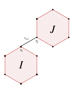
 minimization problem.
 packing of discs. This means that there are also two chiral densest
  packings of all
 and
and  group. Even though they belong to different crystal systems—triclinic for
  ,
,  , and
, and  . Here’s a snapshot of what this packing looks like:
 ,
,  , and
, and  . Check out the illustration below of the densest packing configuration:
 ,
, 
 , highlighting its sixfold rotational symmetry and mirror reflection properties.